T Stellaria palustris Retz. - Vaccinium myrtillus L.
T.1 Stellaria palustris Retz.
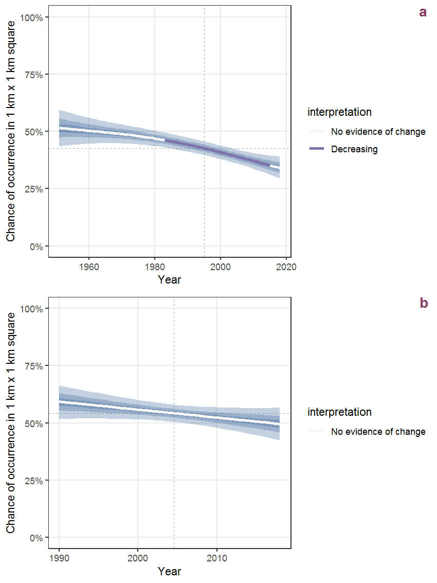
Figure T.1: Effect of year on the probability of Stellaria palustris Retz. presence in 1 km x 1 km squares where the species has been observed at least once. The fitted line shows the sum of the overall mean (the intercept), a conditional effect of list-length equal to 130 and the year-smoother. The vertical dashed lines indicate the year(s) where the year-smoother is zero. The 95% confidence band is shown in grey (including the variability around the intercept and the smoother). a: 1950 - 2018, b: 1990 - 2018.
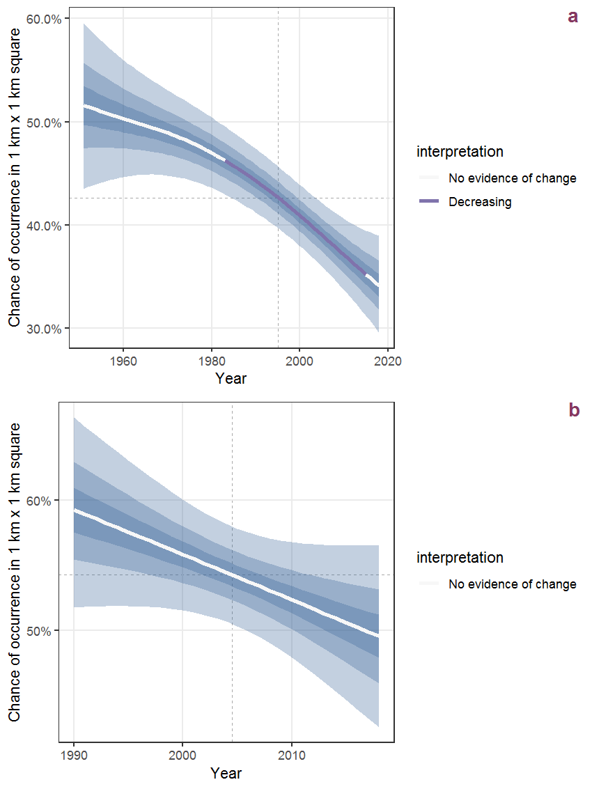
Figure T.2: The same as T.1, but the vertical axis is scaled to the range of the predicted values such that relative changes can be seen more easily. a: 1950 - 2018, b: 1990 - 2018.
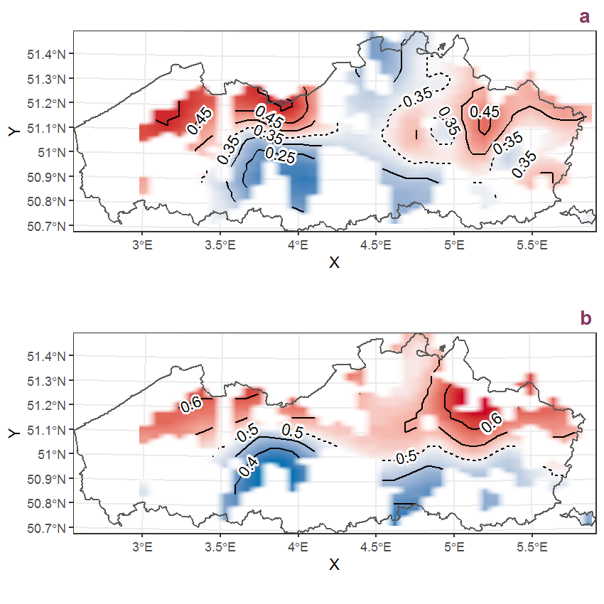
Figure T.3: Visualisation of the spatial smooth effect on the probability of Stellaria palustris Retz. presence in 1 km x 1 km squares where the species has been observed at least once. The probabilities (values on the contour lines) are conditional on the final year of observation and a list-length equal to 130. The dashed contour line demarcates zones where the species is expected to be more prevalent (red shades) from zones where the species is less prevalent (blue shades). a: 1950 - 2018, b: 1990 - 2018.
T.2 Stellaria alsine Grimm
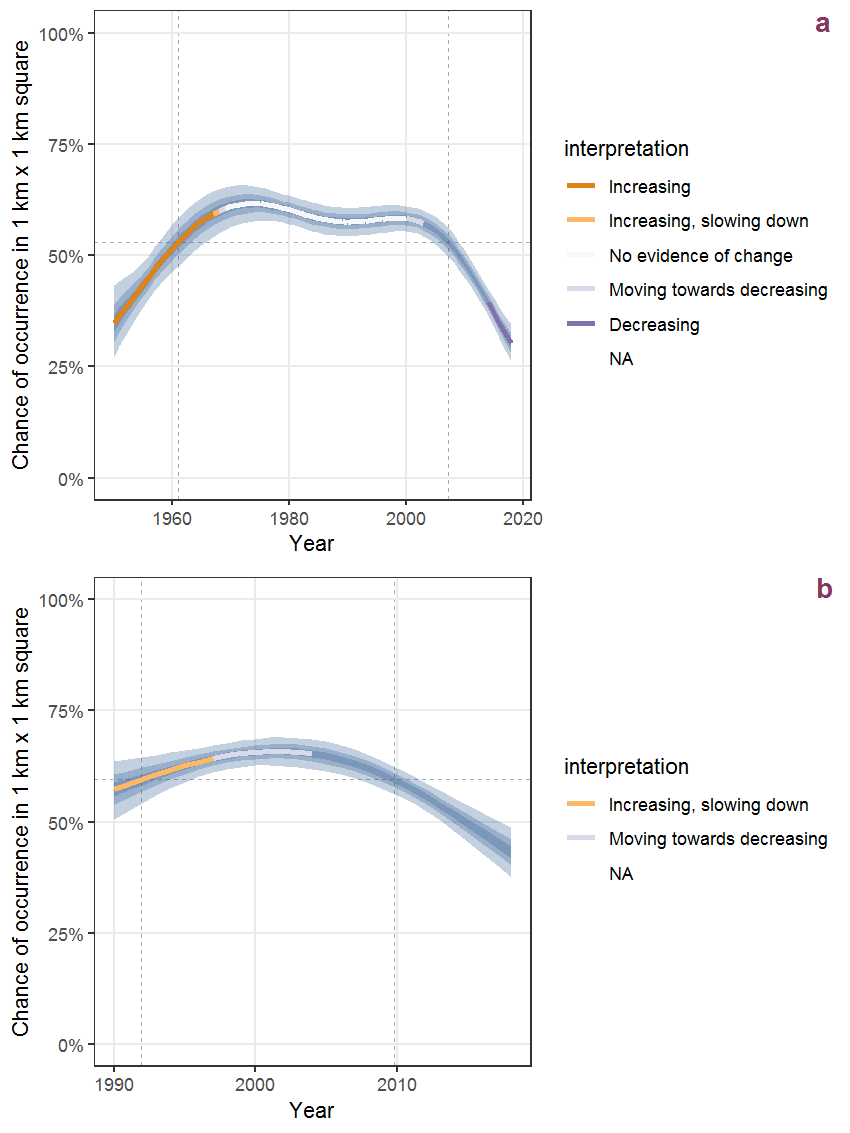
Figure T.4: Effect of year on the probability of Stellaria alsine Grimm presence in 1 km x 1 km squares where the species has been observed at least once. The fitted line shows the sum of the overall mean (the intercept), a conditional effect of list-length equal to 130 and the year-smoother. The vertical dashed lines indicate the year(s) where the year-smoother is zero. The 95% confidence band is shown in grey (including the variability around the intercept and the smoother). a: 1950 - 2018, b: 1990 - 2018.
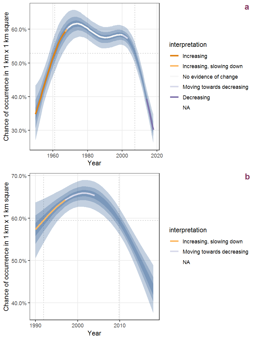
Figure T.5: The same as T.4, but the vertical axis is scaled to the range of the predicted values such that relative changes can be seen more easily. a: 1950 - 2018, b: 1990 - 2018.
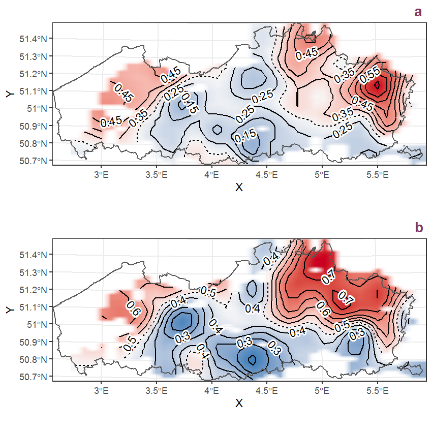
Figure T.6: Visualisation of the spatial smooth effect on the probability of Stellaria alsine Grimm presence in 1 km x 1 km squares where the species has been observed at least once. The probabilities (values on the contour lines) are conditional on the final year of observation and a list-length equal to 130. The dashed contour line demarcates zones where the species is expected to be more prevalent (red shades) from zones where the species is less prevalent (blue shades). a: 1950 - 2018, b: 1990 - 2018.
T.3 Succisa pratensis Moench
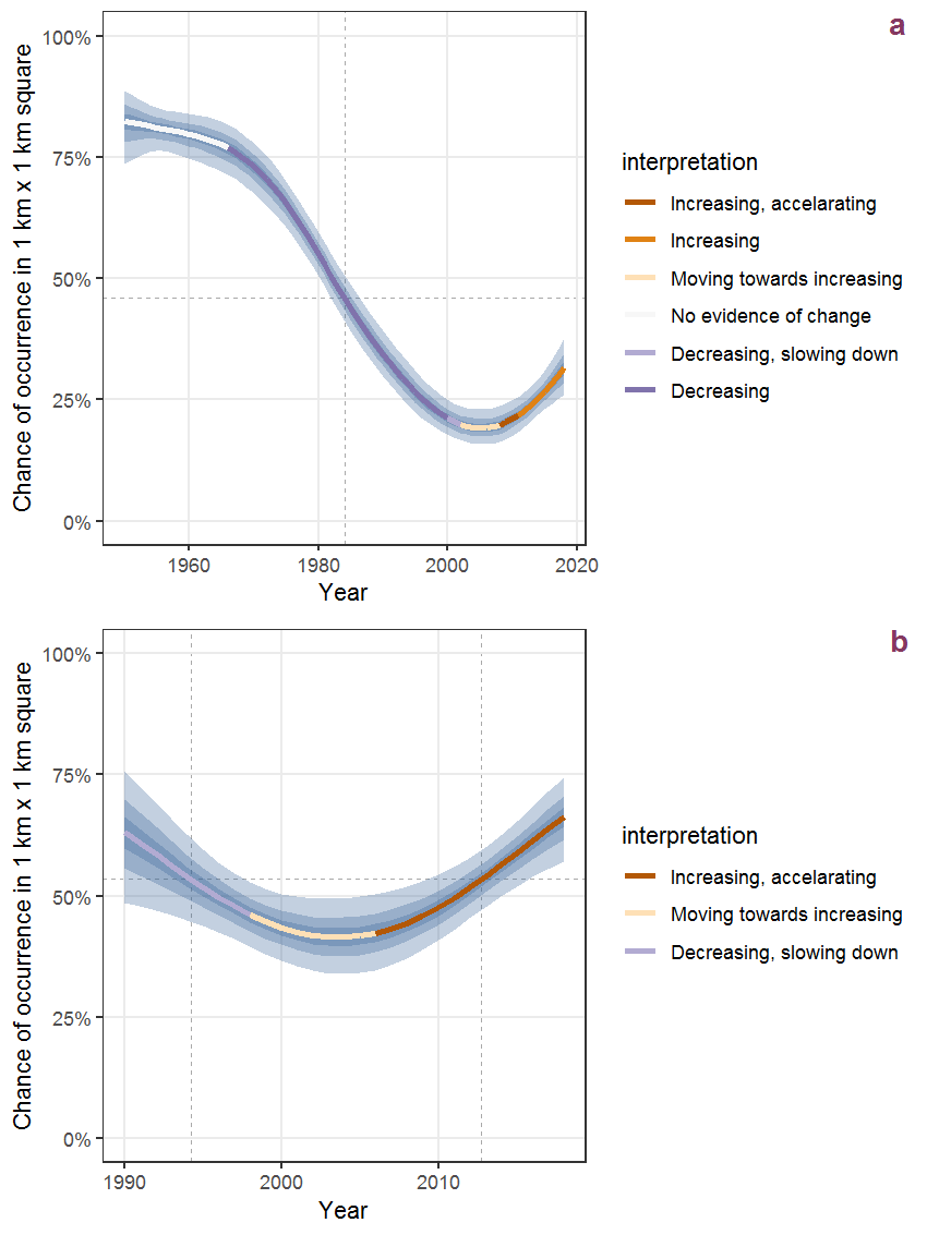
Figure T.7: Effect of year on the probability of Succisa pratensis Moench presence in 1 km x 1 km squares where the species has been observed at least once. The fitted line shows the sum of the overall mean (the intercept), a conditional effect of list-length equal to 130 and the year-smoother. The vertical dashed lines indicate the year(s) where the year-smoother is zero. The 95% confidence band is shown in grey (including the variability around the intercept and the smoother). a: 1950 - 2018, b: 1990 - 2018.
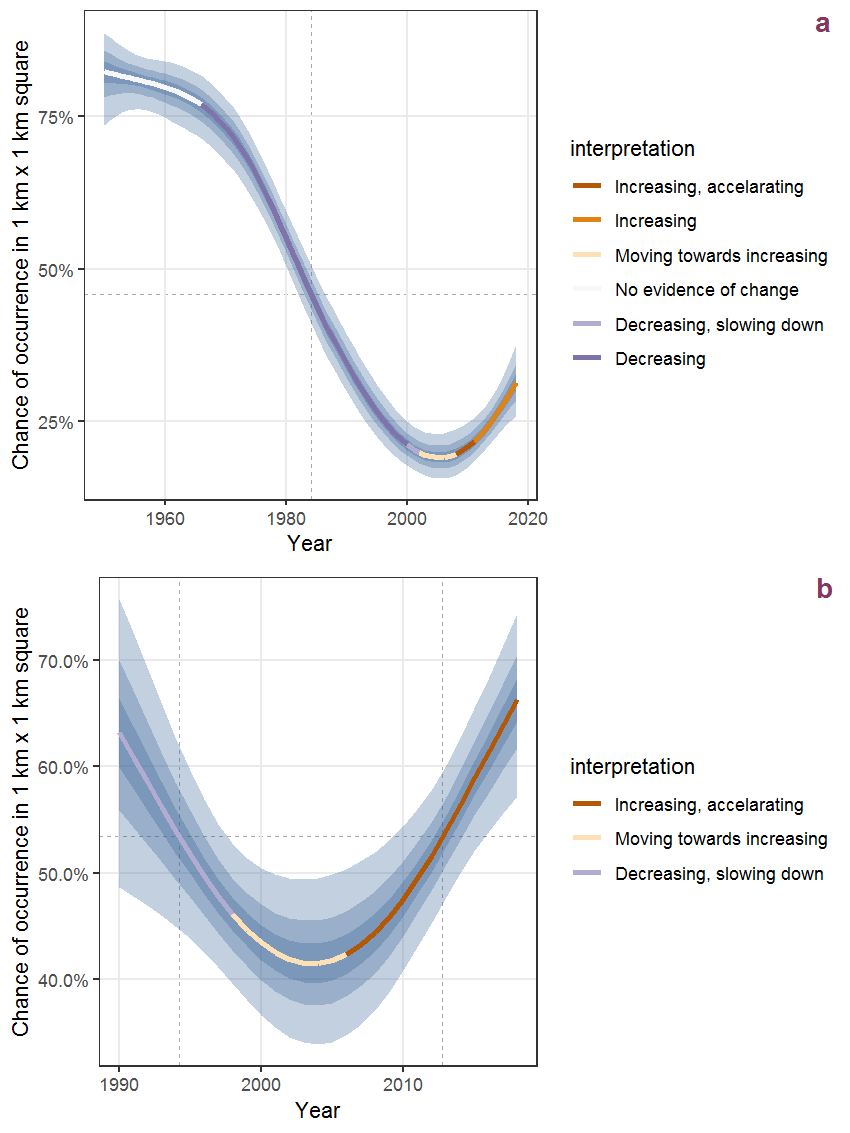
Figure T.8: The same as T.7, but the vertical axis is scaled to the range of the predicted values such that relative changes can be seen more easily. a: 1950 - 2018, b: 1990 - 2018.
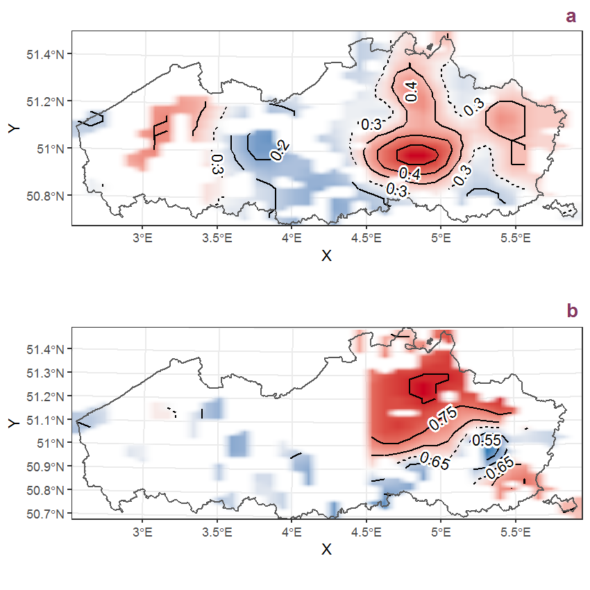
Figure T.9: Visualisation of the spatial smooth effect on the probability of Succisa pratensis Moench presence in 1 km x 1 km squares where the species has been observed at least once. The probabilities (values on the contour lines) are conditional on the final year of observation and a list-length equal to 130. The dashed contour line demarcates zones where the species is expected to be more prevalent (red shades) from zones where the species is less prevalent (blue shades). a: 1950 - 2018, b: 1990 - 2018.
T.4 Symphytum officinale L.
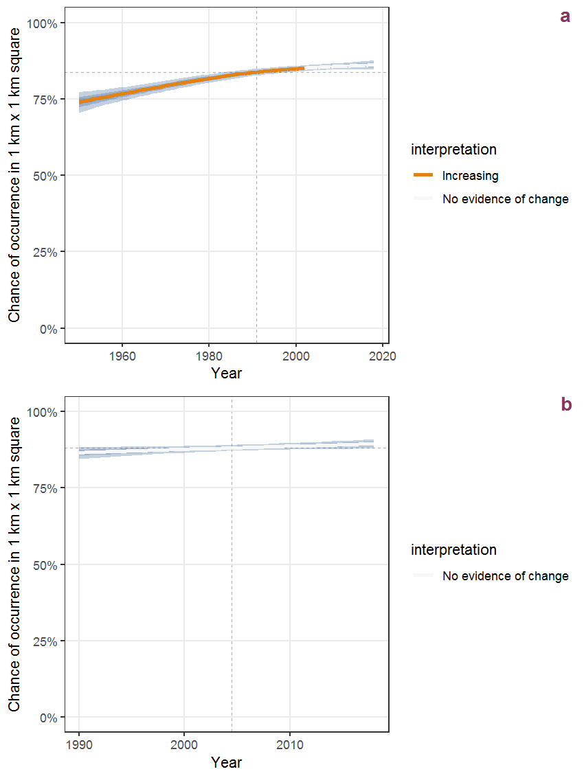
Figure T.10: Effect of year on the probability of Symphytum officinale L. presence in 1 km x 1 km squares where the species has been observed at least once. The fitted line shows the sum of the overall mean (the intercept), a conditional effect of list-length equal to 130 and the year-smoother. The vertical dashed lines indicate the year(s) where the year-smoother is zero. The 95% confidence band is shown in grey (including the variability around the intercept and the smoother). a: 1950 - 2018, b: 1990 - 2018.
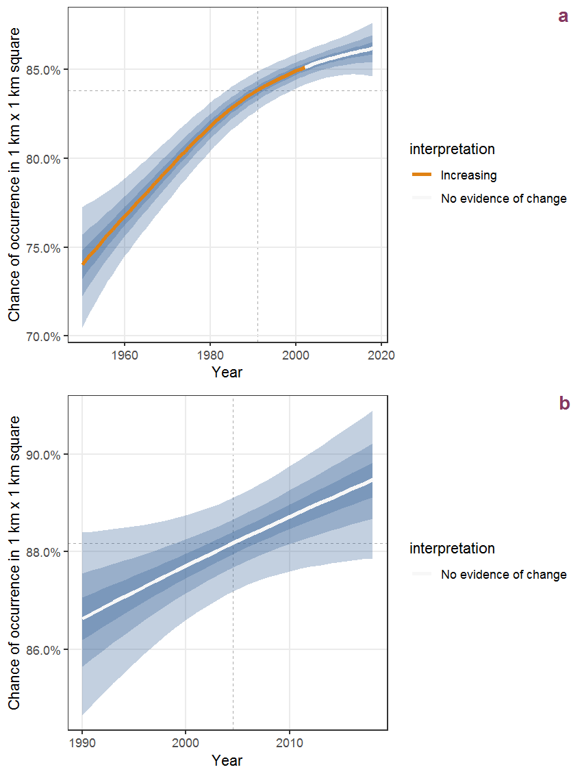
Figure T.11: The same as T.10, but the vertical axis is scaled to the range of the predicted values such that relative changes can be seen more easily. a: 1950 - 2018, b: 1990 - 2018.
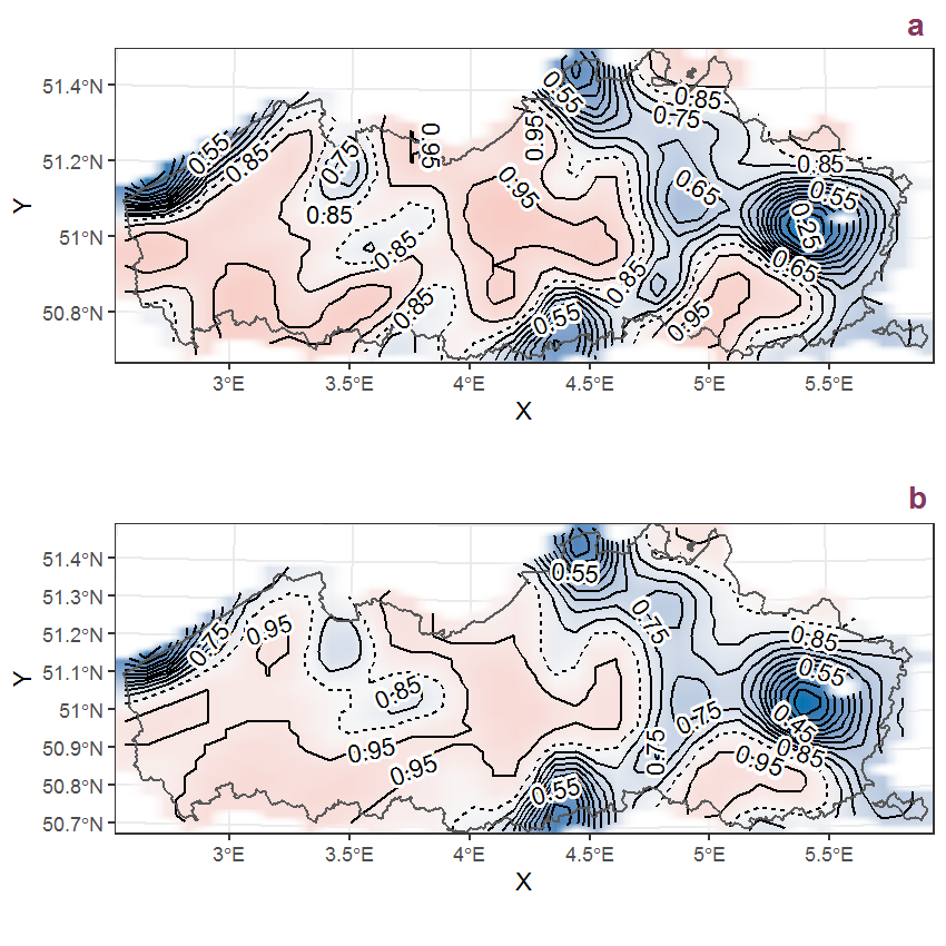
Figure T.12: Visualisation of the spatial smooth effect on the probability of Symphytum officinale L. presence in 1 km x 1 km squares where the species has been observed at least once. The probabilities (values on the contour lines) are conditional on the final year of observation and a list-length equal to 130. The dashed contour line demarcates zones where the species is expected to be more prevalent (red shades) from zones where the species is less prevalent (blue shades). a: 1950 - 2018, b: 1990 - 2018.
T.5 Symphoricarpos albus (L.) S.F. Blake
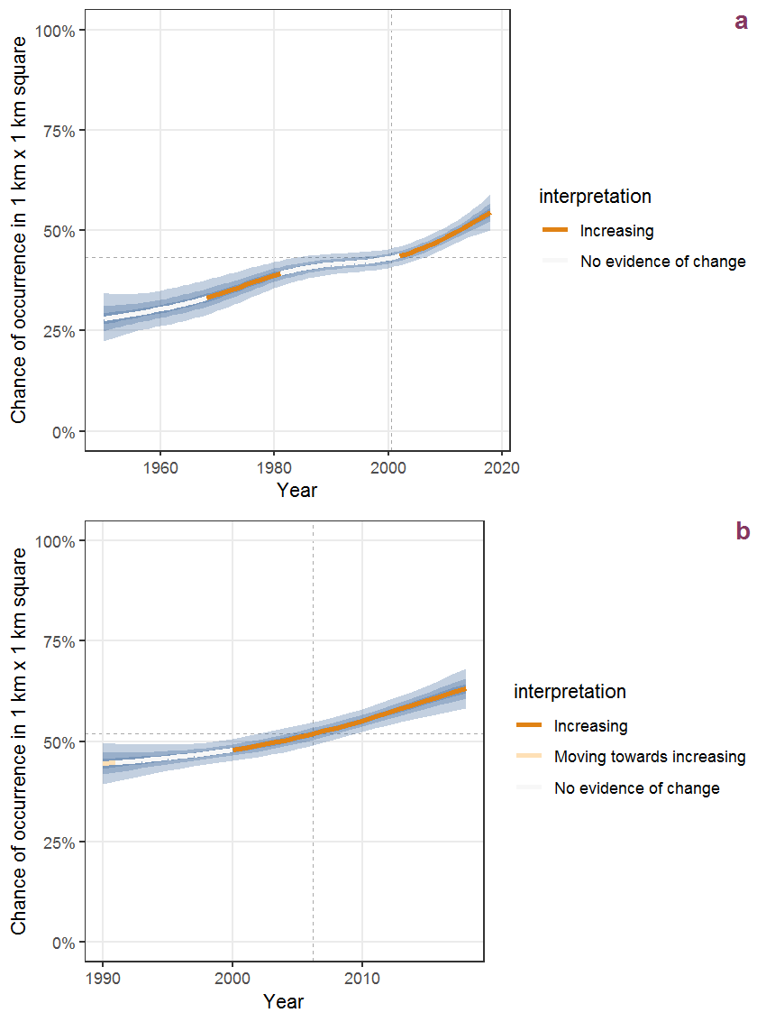
Figure T.13: Effect of year on the probability of Symphoricarpos albus (L.) S.F. Blake presence in 1 km x 1 km squares where the species has been observed at least once. The fitted line shows the sum of the overall mean (the intercept), a conditional effect of list-length equal to 130 and the year-smoother. The vertical dashed lines indicate the year(s) where the year-smoother is zero. The 95% confidence band is shown in grey (including the variability around the intercept and the smoother). a: 1950 - 2018, b: 1990 - 2018.
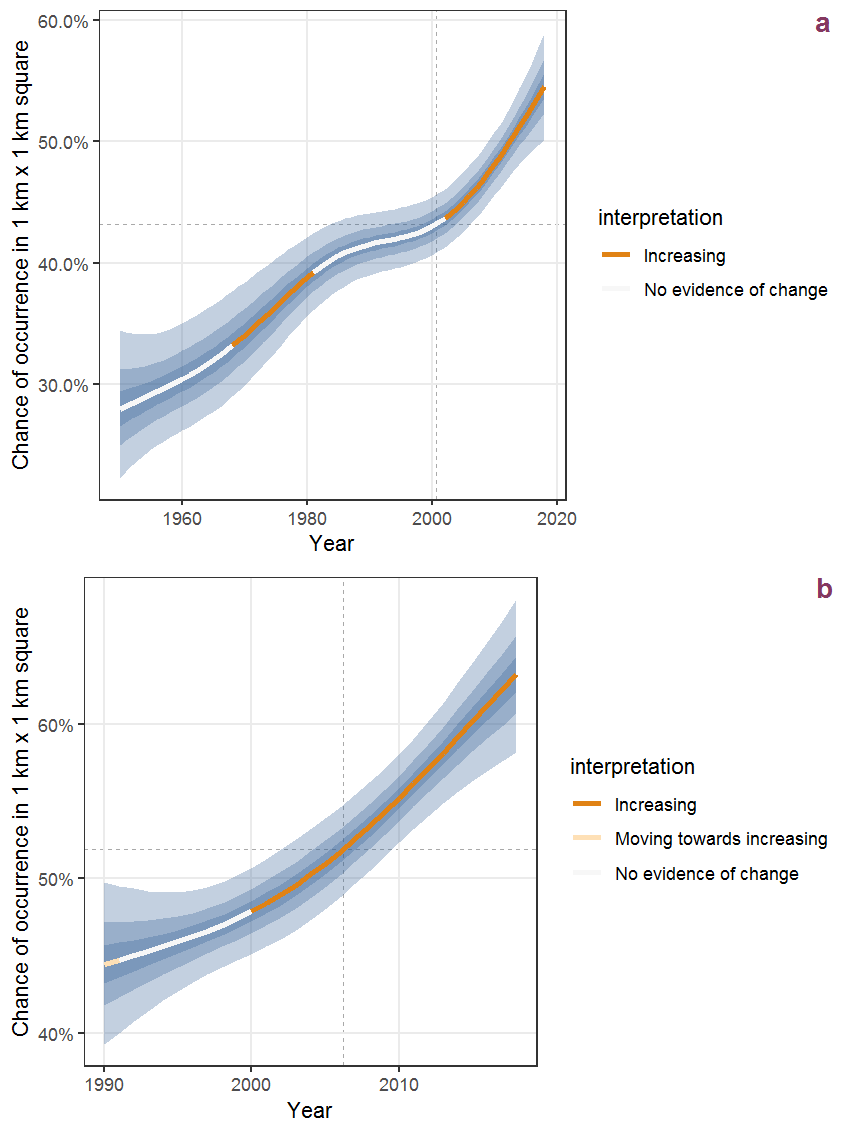
Figure T.14: The same as T.13, but the vertical axis is scaled to the range of the predicted values such that relative changes can be seen more easily. a: 1950 - 2018, b: 1990 - 2018.
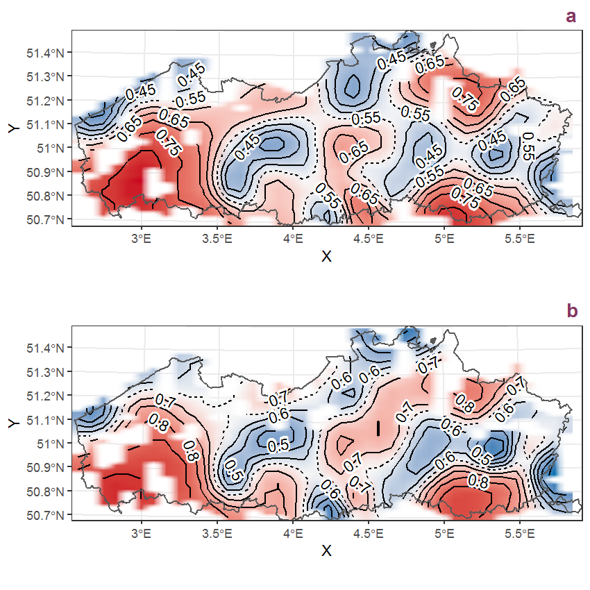
Figure T.15: Visualisation of the spatial smooth effect on the probability of Symphoricarpos albus (L.) S.F. Blake presence in 1 km x 1 km squares where the species has been observed at least once. The probabilities (values on the contour lines) are conditional on the final year of observation and a list-length equal to 130. The dashed contour line demarcates zones where the species is expected to be more prevalent (red shades) from zones where the species is less prevalent (blue shades). a: 1950 - 2018, b: 1990 - 2018.
T.6 Tanacetum parthenium (L.) Schultz-Bip.
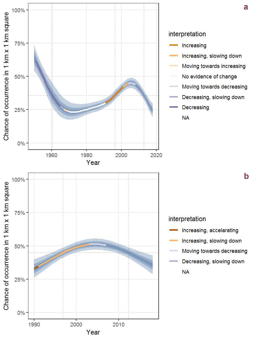
Figure T.16: Effect of year on the probability of Tanacetum parthenium (L.) Schultz-Bip. presence in 1 km x 1 km squares where the species has been observed at least once. The fitted line shows the sum of the overall mean (the intercept), a conditional effect of list-length equal to 130 and the year-smoother. The vertical dashed lines indicate the year(s) where the year-smoother is zero. The 95% confidence band is shown in grey (including the variability around the intercept and the smoother). a: 1950 - 2018, b: 1990 - 2018.
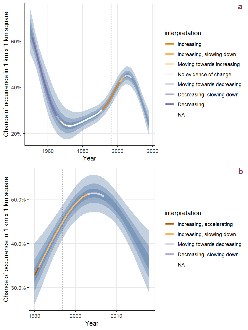
Figure T.17: The same as T.16, but the vertical axis is scaled to the range of the predicted values such that relative changes can be seen more easily. a: 1950 - 2018, b: 1990 - 2018.
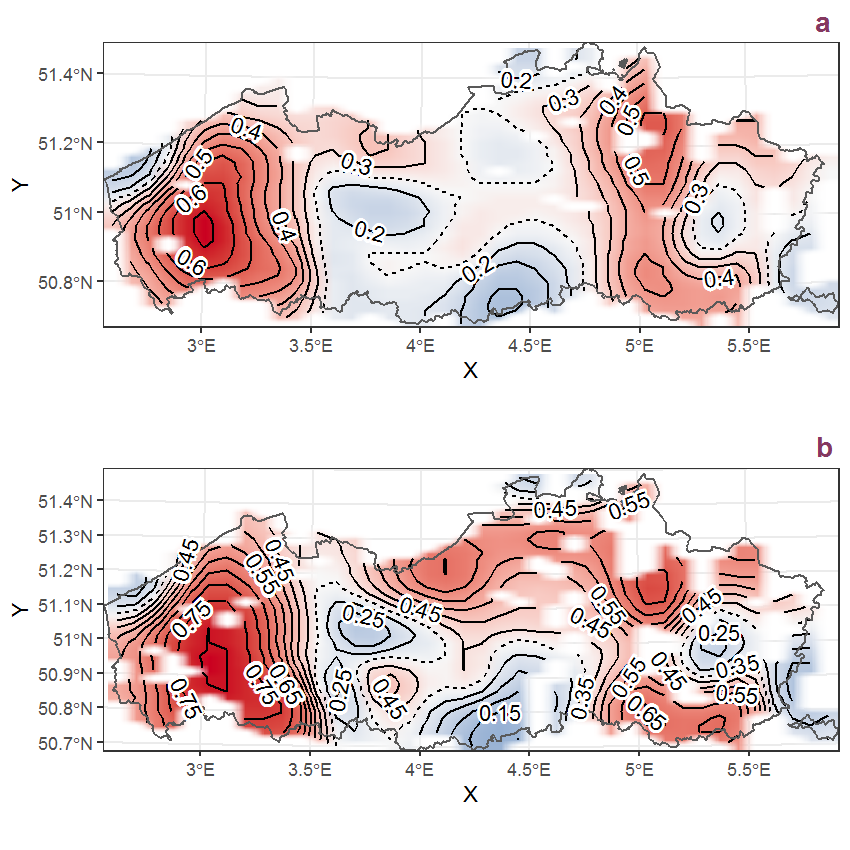
Figure T.18: Visualisation of the spatial smooth effect on the probability of Tanacetum parthenium (L.) Schultz-Bip. presence in 1 km x 1 km squares where the species has been observed at least once. The probabilities (values on the contour lines) are conditional on the final year of observation and a list-length equal to 130. The dashed contour line demarcates zones where the species is expected to be more prevalent (red shades) from zones where the species is less prevalent (blue shades). a: 1950 - 2018, b: 1990 - 2018.
T.7 Tanacetum vulgare L.
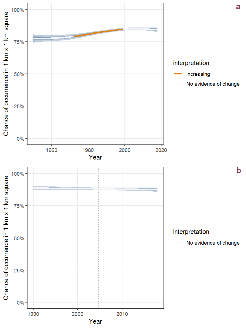
Figure T.19: Effect of year on the probability of Tanacetum vulgare L. presence in 1 km x 1 km squares where the species has been observed at least once. The fitted line shows the sum of the overall mean (the intercept), a conditional effect of list-length equal to 130 and the year-smoother. The vertical dashed lines indicate the year(s) where the year-smoother is zero. The 95% confidence band is shown in grey (including the variability around the intercept and the smoother). a: 1950 - 2018, b: 1990 - 2018.
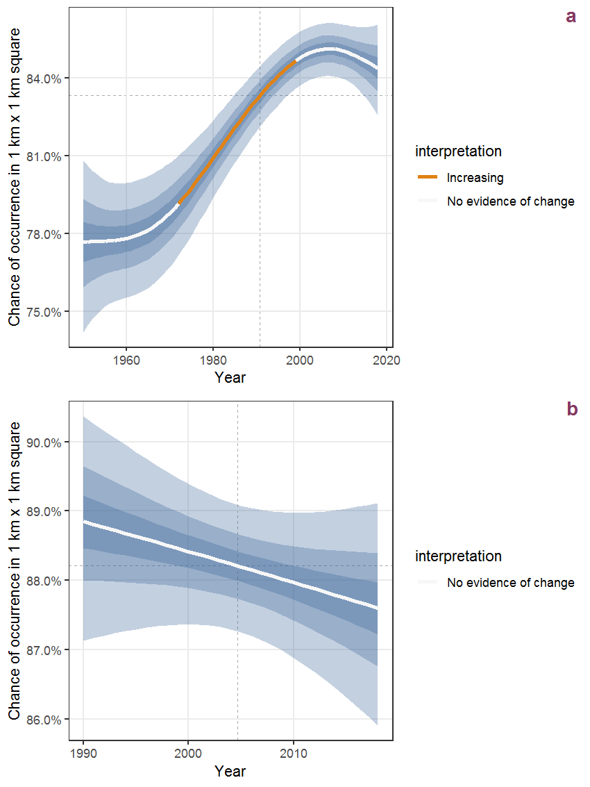
Figure T.20: The same as T.19, but the vertical axis is scaled to the range of the predicted values such that relative changes can be seen more easily. a: 1950 - 2018, b: 1990 - 2018.
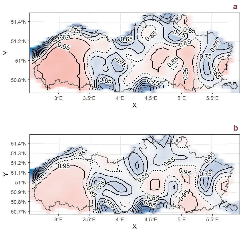
Figure T.21: Visualisation of the spatial smooth effect on the probability of Tanacetum vulgare L. presence in 1 km x 1 km squares where the species has been observed at least once. The probabilities (values on the contour lines) are conditional on the final year of observation and a list-length equal to 130. The dashed contour line demarcates zones where the species is expected to be more prevalent (red shades) from zones where the species is less prevalent (blue shades). a: 1950 - 2018, b: 1990 - 2018.
T.8 Taxus baccata L.
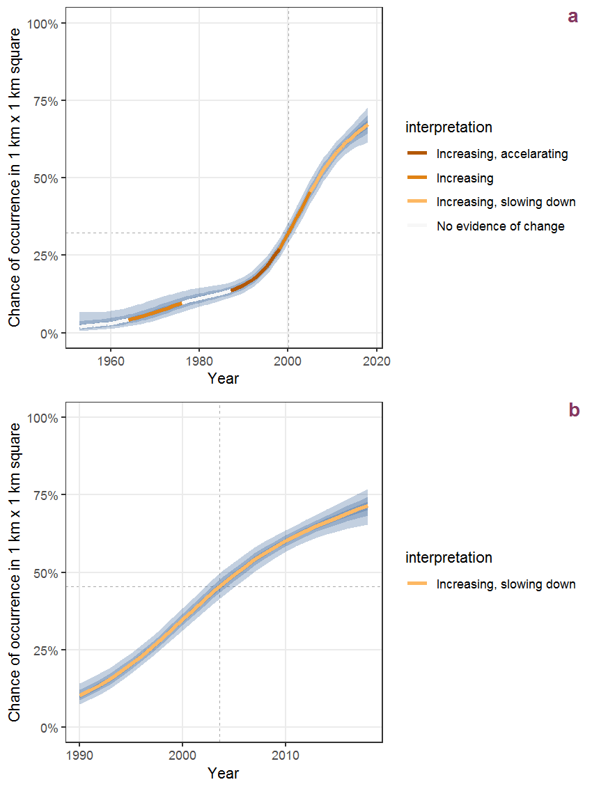
Figure T.22: Effect of year on the probability of Taxus baccata L. presence in 1 km x 1 km squares where the species has been observed at least once. The fitted line shows the sum of the overall mean (the intercept), a conditional effect of list-length equal to 130 and the year-smoother. The vertical dashed lines indicate the year(s) where the year-smoother is zero. The 95% confidence band is shown in grey (including the variability around the intercept and the smoother). a: 1950 - 2018, b: 1990 - 2018.
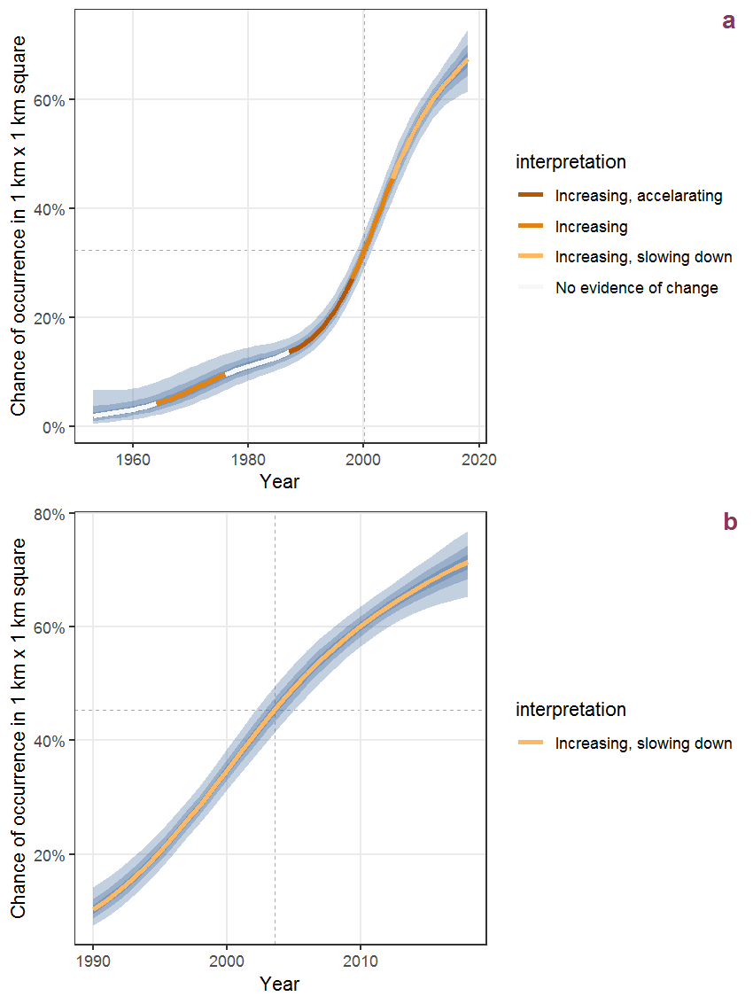
Figure T.23: The same as T.22, but the vertical axis is scaled to the range of the predicted values such that relative changes can be seen more easily. a: 1950 - 2018, b: 1990 - 2018.
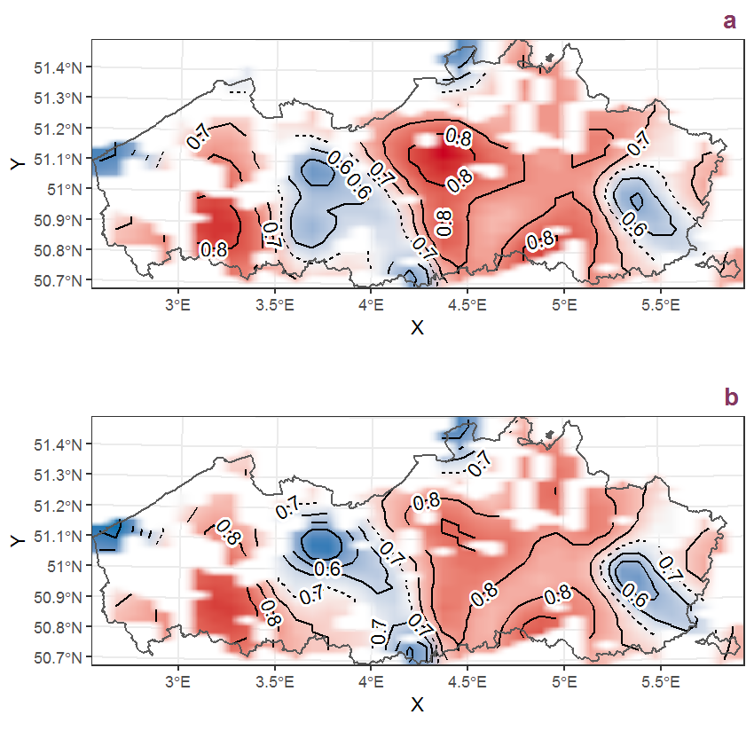
Figure T.24: Visualisation of the spatial smooth effect on the probability of Taxus baccata L. presence in 1 km x 1 km squares where the species has been observed at least once. The probabilities (values on the contour lines) are conditional on the final year of observation and a list-length equal to 130. The dashed contour line demarcates zones where the species is expected to be more prevalent (red shades) from zones where the species is less prevalent (blue shades). a: 1950 - 2018, b: 1990 - 2018.
T.9 Teucrium scorodonia L.
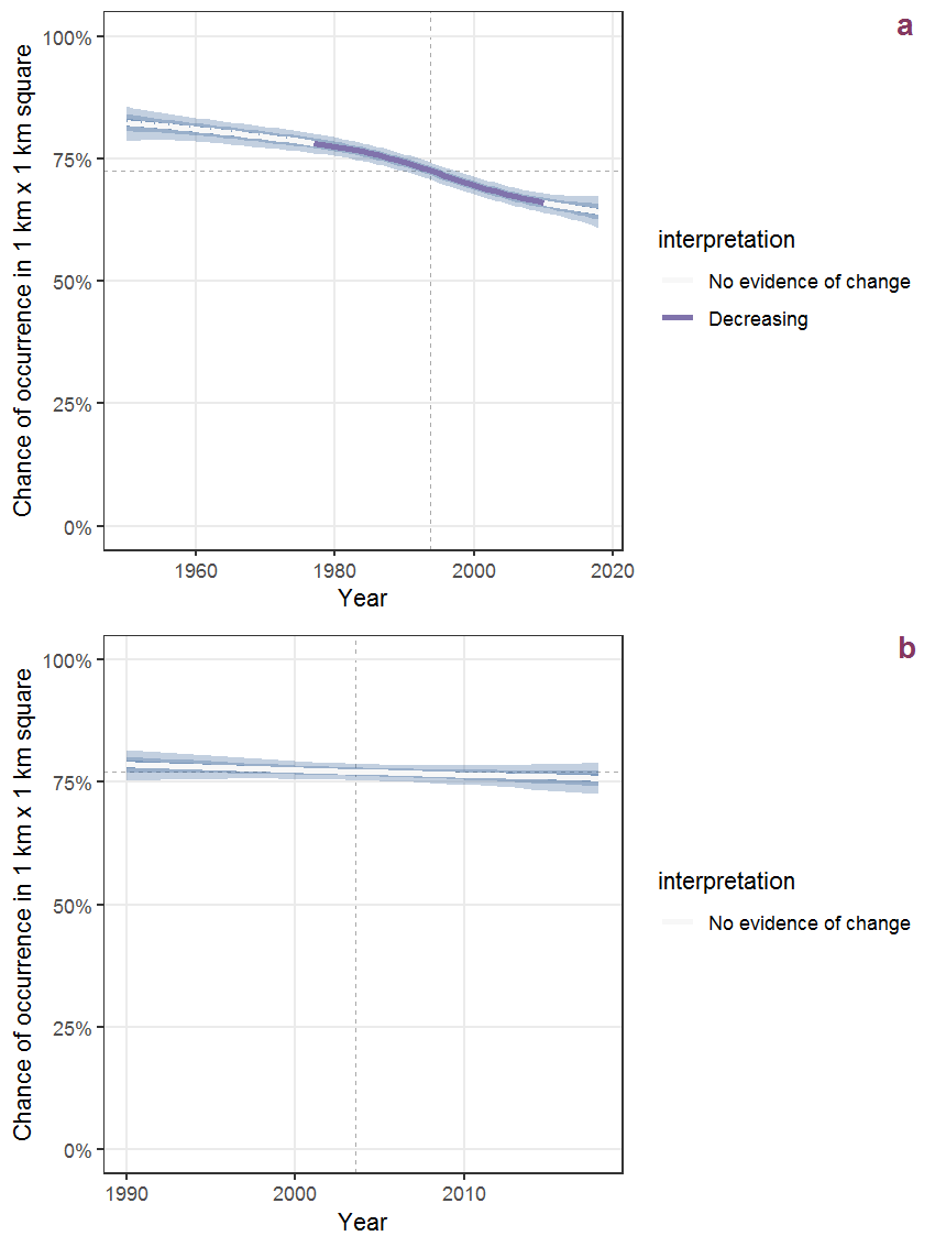
Figure T.25: Effect of year on the probability of Teucrium scorodonia L. presence in 1 km x 1 km squares where the species has been observed at least once. The fitted line shows the sum of the overall mean (the intercept), a conditional effect of list-length equal to 130 and the year-smoother. The vertical dashed lines indicate the year(s) where the year-smoother is zero. The 95% confidence band is shown in grey (including the variability around the intercept and the smoother). a: 1950 - 2018, b: 1990 - 2018.
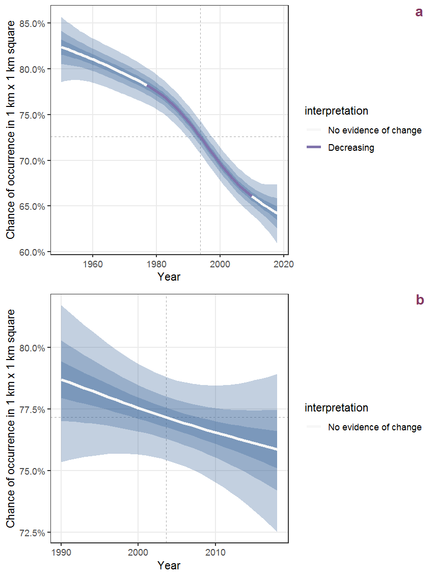
Figure T.26: The same as T.25, but the vertical axis is scaled to the range of the predicted values such that relative changes can be seen more easily. a: 1950 - 2018, b: 1990 - 2018.
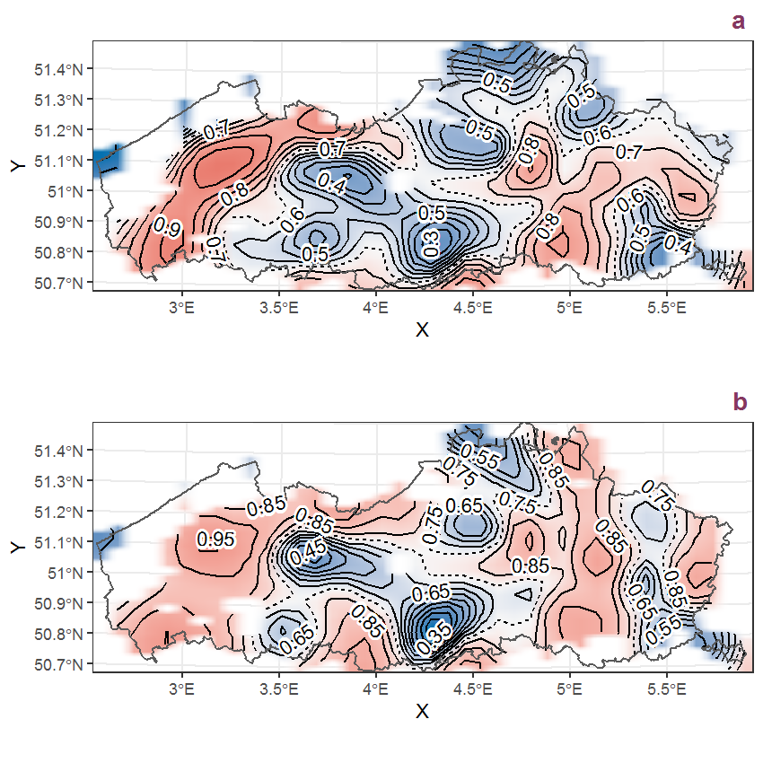
Figure T.27: Visualisation of the spatial smooth effect on the probability of Teucrium scorodonia L. presence in 1 km x 1 km squares where the species has been observed at least once. The probabilities (values on the contour lines) are conditional on the final year of observation and a list-length equal to 130. The dashed contour line demarcates zones where the species is expected to be more prevalent (red shades) from zones where the species is less prevalent (blue shades). a: 1950 - 2018, b: 1990 - 2018.
T.10 Thalictrum flavum L.
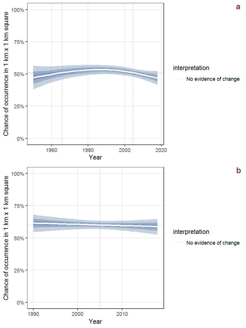
Figure T.28: Effect of year on the probability of Thalictrum flavum L. presence in 1 km x 1 km squares where the species has been observed at least once. The fitted line shows the sum of the overall mean (the intercept), a conditional effect of list-length equal to 130 and the year-smoother. The vertical dashed lines indicate the year(s) where the year-smoother is zero. The 95% confidence band is shown in grey (including the variability around the intercept and the smoother). a: 1950 - 2018, b: 1990 - 2018.
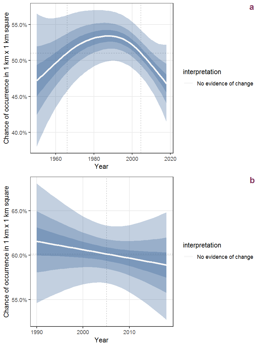
Figure T.29: The same as T.28, but the vertical axis is scaled to the range of the predicted values such that relative changes can be seen more easily. a: 1950 - 2018, b: 1990 - 2018.
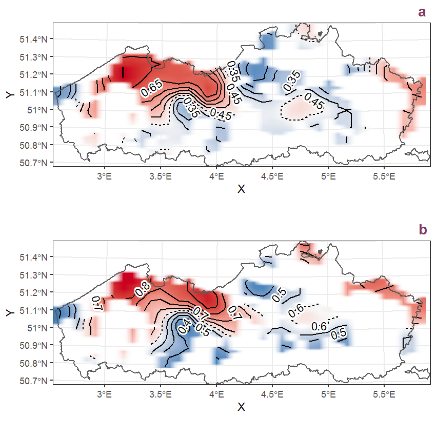
Figure T.30: Visualisation of the spatial smooth effect on the probability of Thalictrum flavum L. presence in 1 km x 1 km squares where the species has been observed at least once. The probabilities (values on the contour lines) are conditional on the final year of observation and a list-length equal to 130. The dashed contour line demarcates zones where the species is expected to be more prevalent (red shades) from zones where the species is less prevalent (blue shades). a: 1950 - 2018, b: 1990 - 2018.
T.11 Thlaspi arvense L.
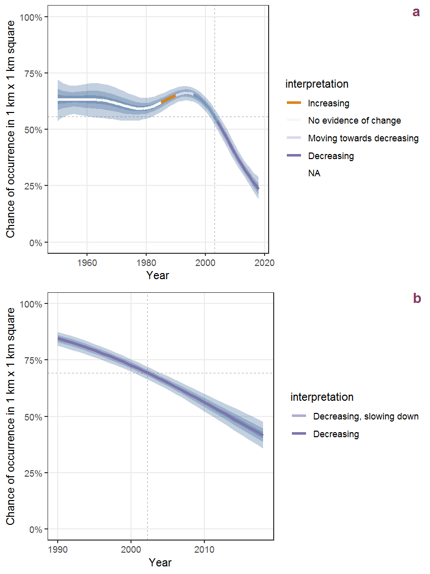
Figure T.31: Effect of year on the probability of Thlaspi arvense L. presence in 1 km x 1 km squares where the species has been observed at least once. The fitted line shows the sum of the overall mean (the intercept), a conditional effect of list-length equal to 130 and the year-smoother. The vertical dashed lines indicate the year(s) where the year-smoother is zero. The 95% confidence band is shown in grey (including the variability around the intercept and the smoother). a: 1950 - 2018, b: 1990 - 2018.
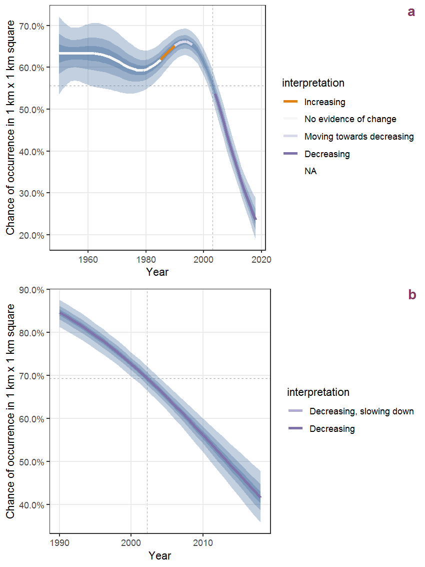
Figure T.32: The same as T.31, but the vertical axis is scaled to the range of the predicted values such that relative changes can be seen more easily. a: 1950 - 2018, b: 1990 - 2018.
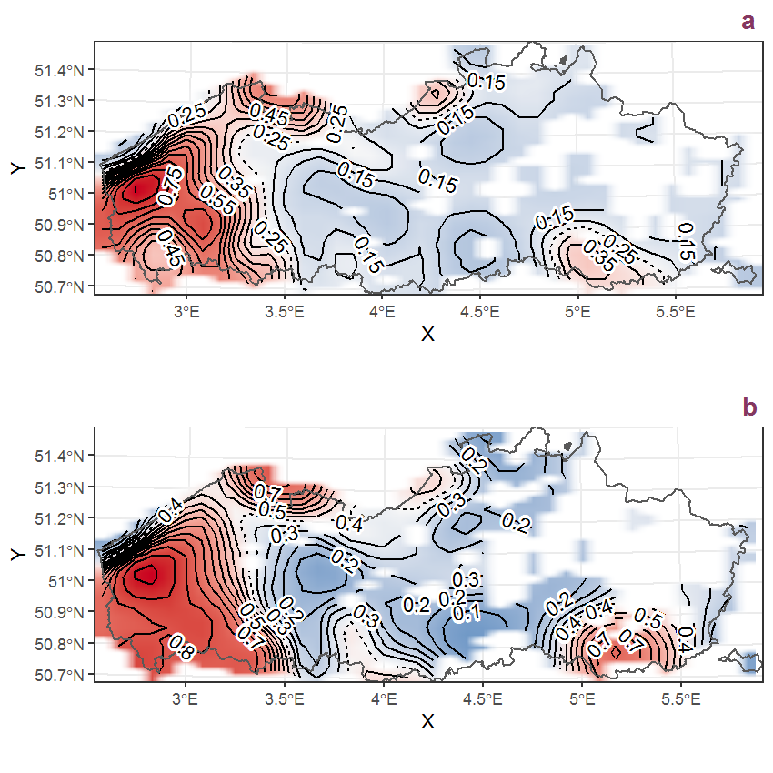
Figure T.33: Visualisation of the spatial smooth effect on the probability of Thlaspi arvense L. presence in 1 km x 1 km squares where the species has been observed at least once. The probabilities (values on the contour lines) are conditional on the final year of observation and a list-length equal to 130. The dashed contour line demarcates zones where the species is expected to be more prevalent (red shades) from zones where the species is less prevalent (blue shades). a: 1950 - 2018, b: 1990 - 2018.
T.12 Thymus pulegioides L.
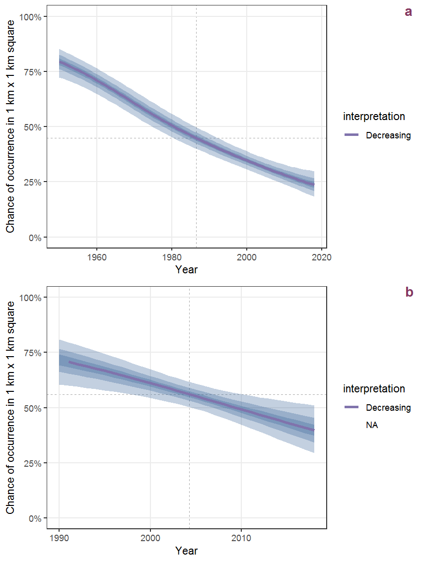
Figure T.34: Effect of year on the probability of Thymus pulegioides L. presence in 1 km x 1 km squares where the species has been observed at least once. The fitted line shows the sum of the overall mean (the intercept), a conditional effect of list-length equal to 130 and the year-smoother. The vertical dashed lines indicate the year(s) where the year-smoother is zero. The 95% confidence band is shown in grey (including the variability around the intercept and the smoother). a: 1950 - 2018, b: 1990 - 2018.
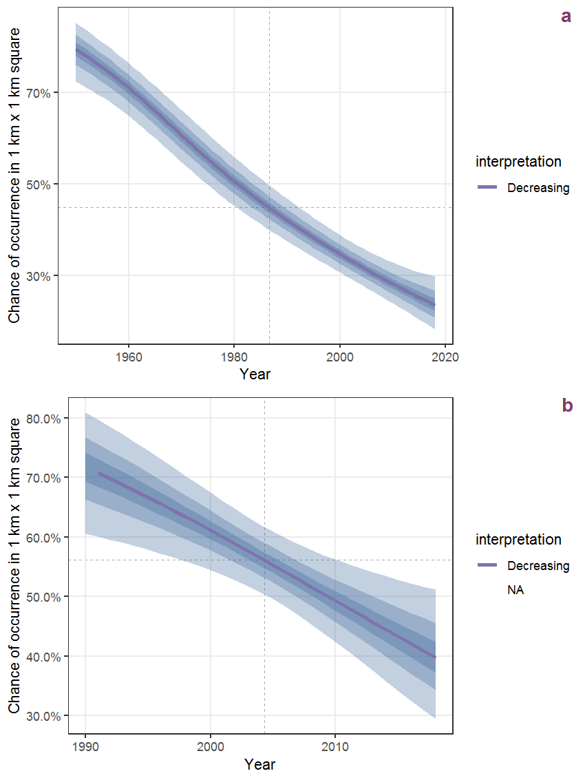
Figure T.35: The same as T.34, but the vertical axis is scaled to the range of the predicted values such that relative changes can be seen more easily. a: 1950 - 2018, b: 1990 - 2018.
## Error in nullGrob(): could not find function "nullGrob"T.13 Tilia cordata Mill.
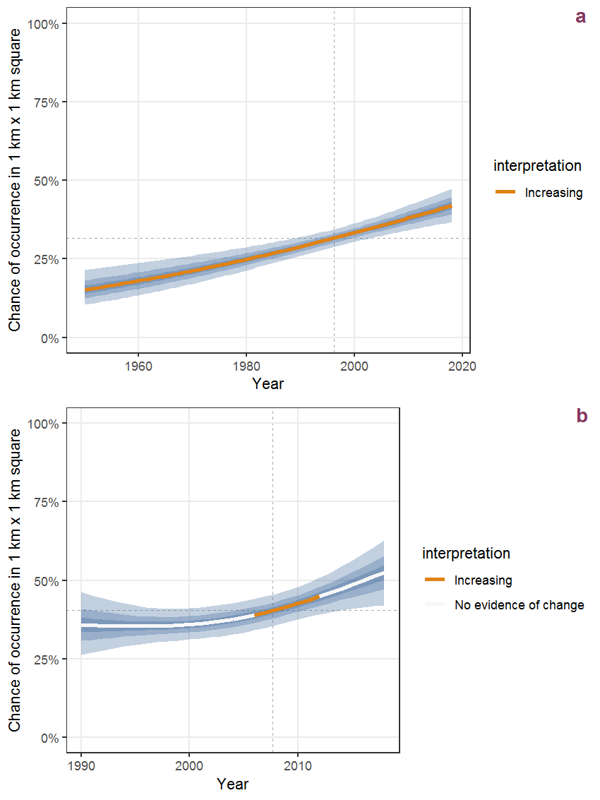
Figure T.36: Effect of year on the probability of Tilia cordata Mill. presence in 1 km x 1 km squares where the species has been observed at least once. The fitted line shows the sum of the overall mean (the intercept), a conditional effect of list-length equal to 130 and the year-smoother. The vertical dashed lines indicate the year(s) where the year-smoother is zero. The 95% confidence band is shown in grey (including the variability around the intercept and the smoother). a: 1950 - 2018, b: 1990 - 2018.
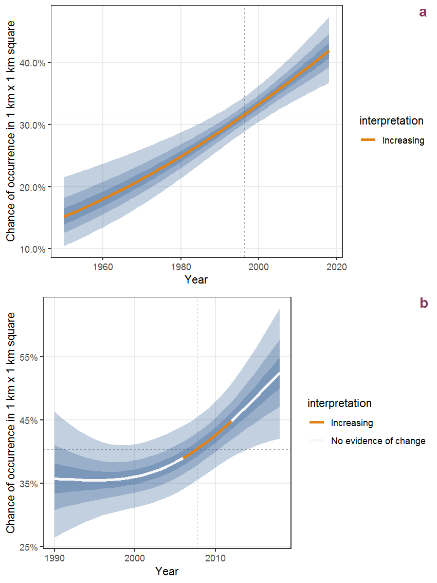
Figure T.37: The same as T.36, but the vertical axis is scaled to the range of the predicted values such that relative changes can be seen more easily. a: 1950 - 2018, b: 1990 - 2018.
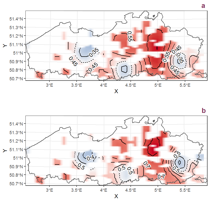
Figure T.38: Visualisation of the spatial smooth effect on the probability of Tilia cordata Mill. presence in 1 km x 1 km squares where the species has been observed at least once. The probabilities (values on the contour lines) are conditional on the final year of observation and a list-length equal to 130. The dashed contour line demarcates zones where the species is expected to be more prevalent (red shades) from zones where the species is less prevalent (blue shades). a: 1950 - 2018, b: 1990 - 2018.
T.14 Tilia platyphyllos Scop. (incl. kruisingen)
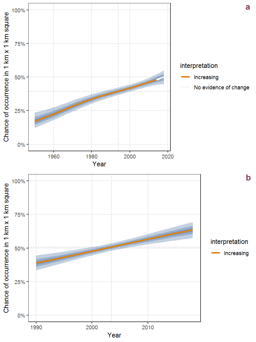
Figure T.39: Effect of year on the probability of Tilia platyphyllos Scop. (incl. kruisingen) presence in 1 km x 1 km squares where the species has been observed at least once. The fitted line shows the sum of the overall mean (the intercept), a conditional effect of list-length equal to 130 and the year-smoother. The vertical dashed lines indicate the year(s) where the year-smoother is zero. The 95% confidence band is shown in grey (including the variability around the intercept and the smoother). a: 1950 - 2018, b: 1990 - 2018.
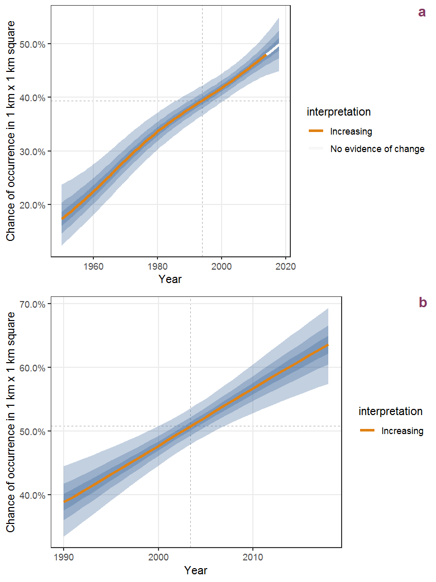
Figure T.40: The same as T.39, but the vertical axis is scaled to the range of the predicted values such that relative changes can be seen more easily. a: 1950 - 2018, b: 1990 - 2018.
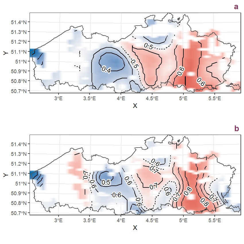
Figure T.41: Visualisation of the spatial smooth effect on the probability of Tilia platyphyllos Scop. (incl. kruisingen) presence in 1 km x 1 km squares where the species has been observed at least once. The probabilities (values on the contour lines) are conditional on the final year of observation and a list-length equal to 130. The dashed contour line demarcates zones where the species is expected to be more prevalent (red shades) from zones where the species is less prevalent (blue shades). a: 1950 - 2018, b: 1990 - 2018.
T.15 Torilis japonica (Houtt.) DC.
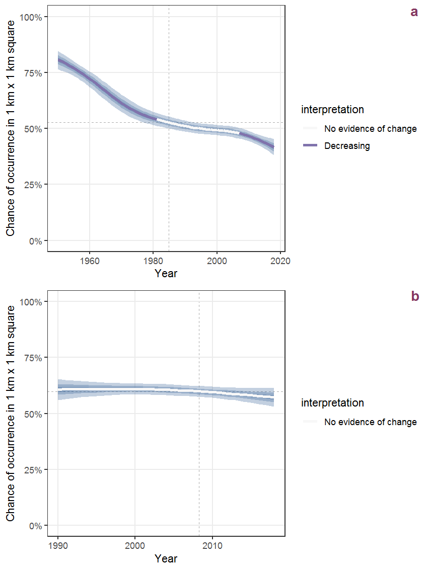
Figure T.42: Effect of year on the probability of Torilis japonica (Houtt.) DC. presence in 1 km x 1 km squares where the species has been observed at least once. The fitted line shows the sum of the overall mean (the intercept), a conditional effect of list-length equal to 130 and the year-smoother. The vertical dashed lines indicate the year(s) where the year-smoother is zero. The 95% confidence band is shown in grey (including the variability around the intercept and the smoother). a: 1950 - 2018, b: 1990 - 2018.
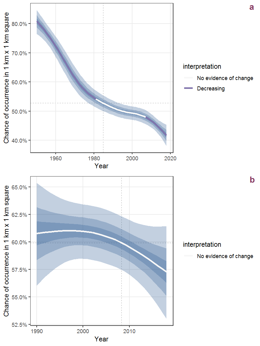
Figure T.43: The same as T.42, but the vertical axis is scaled to the range of the predicted values such that relative changes can be seen more easily. a: 1950 - 2018, b: 1990 - 2018.
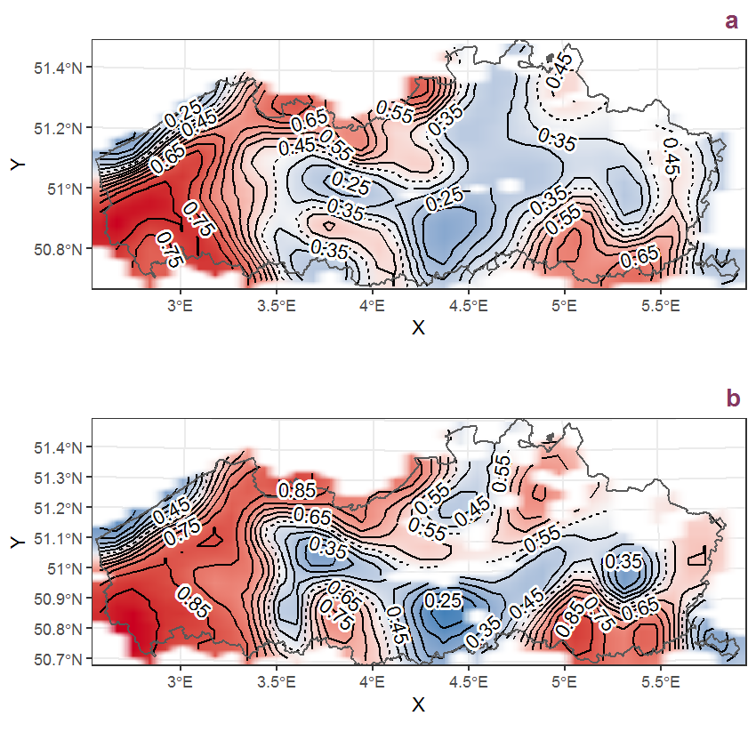
Figure T.44: Visualisation of the spatial smooth effect on the probability of Torilis japonica (Houtt.) DC. presence in 1 km x 1 km squares where the species has been observed at least once. The probabilities (values on the contour lines) are conditional on the final year of observation and a list-length equal to 130. The dashed contour line demarcates zones where the species is expected to be more prevalent (red shades) from zones where the species is less prevalent (blue shades). a: 1950 - 2018, b: 1990 - 2018.
T.16 Tragopogon pratensis L.
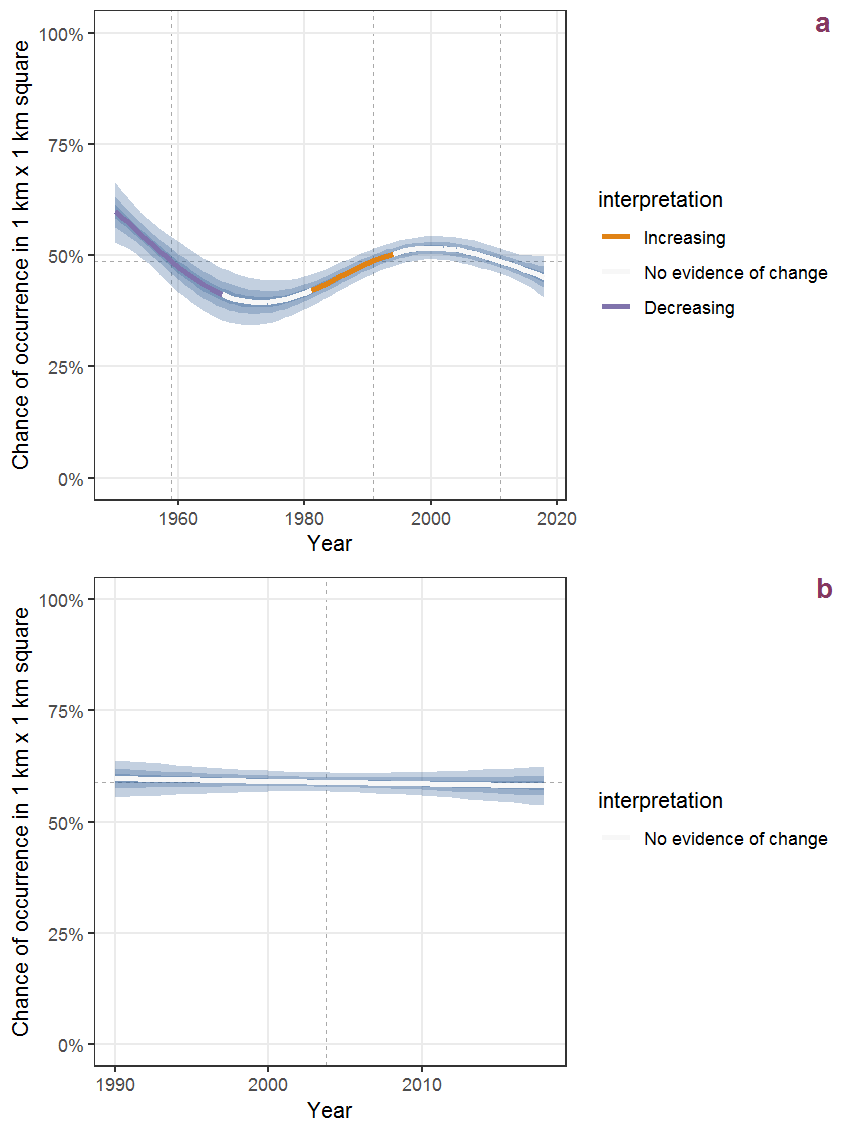
Figure T.45: Effect of year on the probability of Tragopogon pratensis L. presence in 1 km x 1 km squares where the species has been observed at least once. The fitted line shows the sum of the overall mean (the intercept), a conditional effect of list-length equal to 130 and the year-smoother. The vertical dashed lines indicate the year(s) where the year-smoother is zero. The 95% confidence band is shown in grey (including the variability around the intercept and the smoother). a: 1950 - 2018, b: 1990 - 2018.
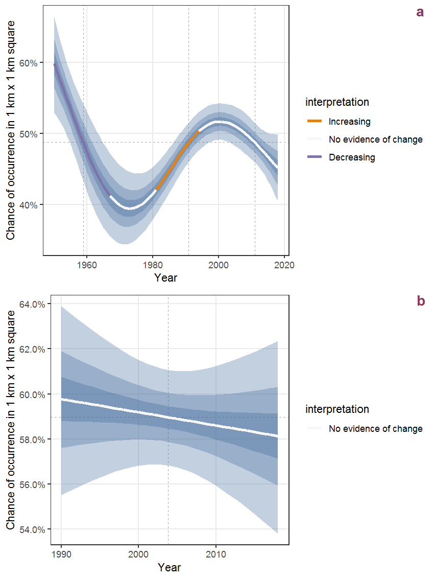
Figure T.46: The same as T.45, but the vertical axis is scaled to the range of the predicted values such that relative changes can be seen more easily. a: 1950 - 2018, b: 1990 - 2018.
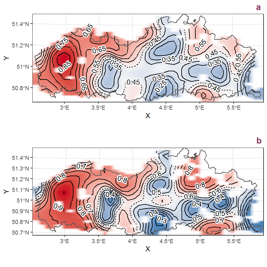
Figure T.47: Visualisation of the spatial smooth effect on the probability of Tragopogon pratensis L. presence in 1 km x 1 km squares where the species has been observed at least once. The probabilities (values on the contour lines) are conditional on the final year of observation and a list-length equal to 130. The dashed contour line demarcates zones where the species is expected to be more prevalent (red shades) from zones where the species is less prevalent (blue shades). a: 1950 - 2018, b: 1990 - 2018.
T.17 Trifolium arvense L.
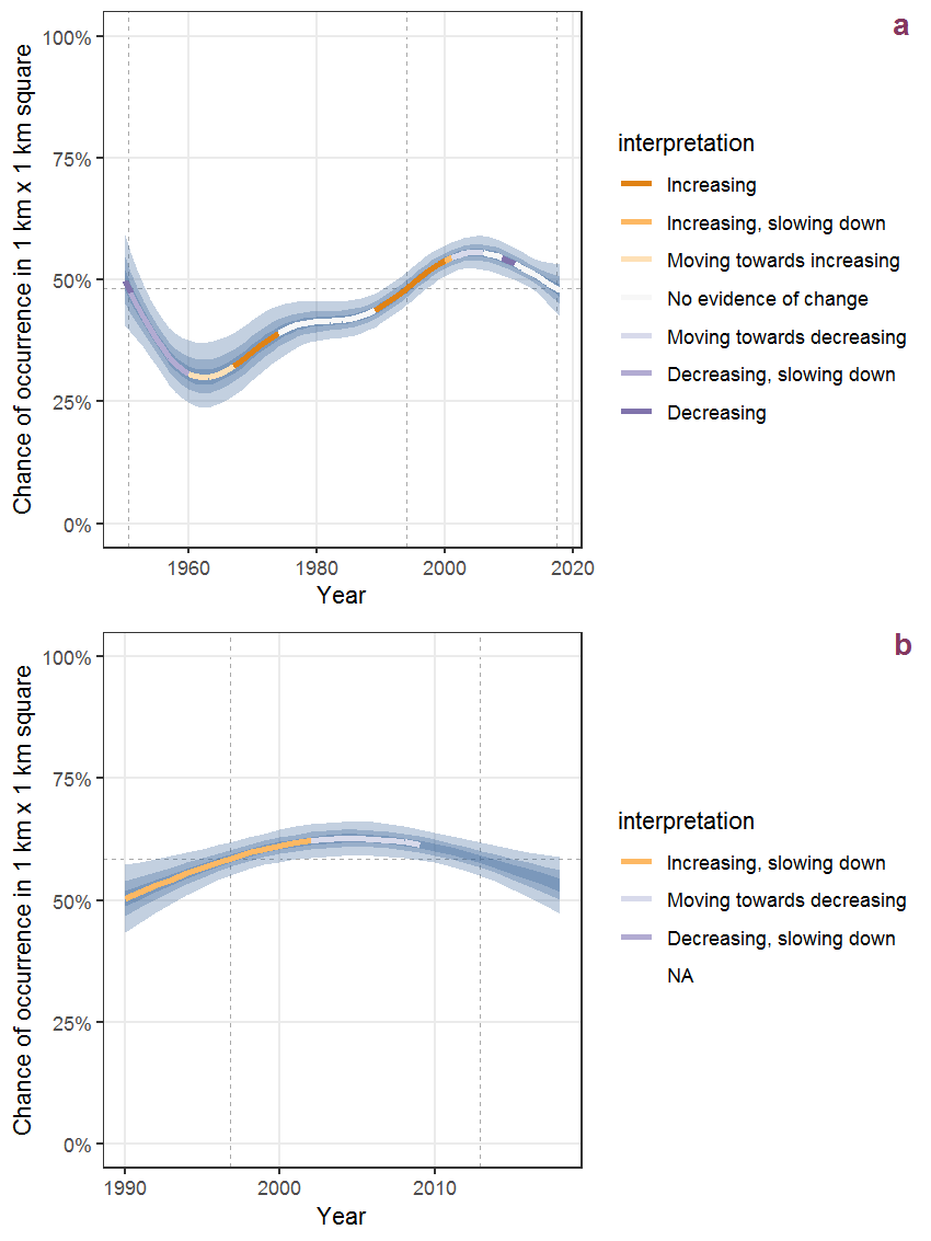
Figure T.48: Effect of year on the probability of Trifolium arvense L. presence in 1 km x 1 km squares where the species has been observed at least once. The fitted line shows the sum of the overall mean (the intercept), a conditional effect of list-length equal to 130 and the year-smoother. The vertical dashed lines indicate the year(s) where the year-smoother is zero. The 95% confidence band is shown in grey (including the variability around the intercept and the smoother). a: 1950 - 2018, b: 1990 - 2018.
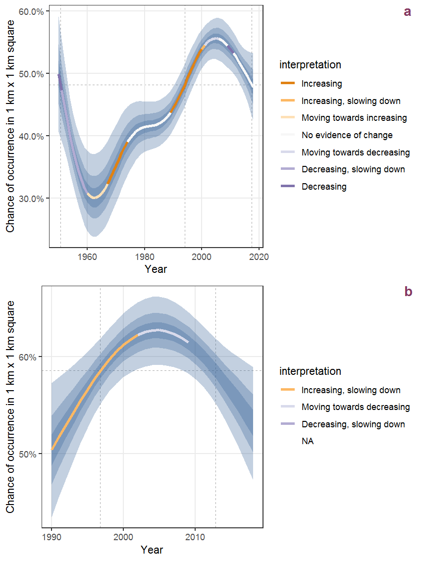
Figure T.49: The same as T.48, but the vertical axis is scaled to the range of the predicted values such that relative changes can be seen more easily. a: 1950 - 2018, b: 1990 - 2018.
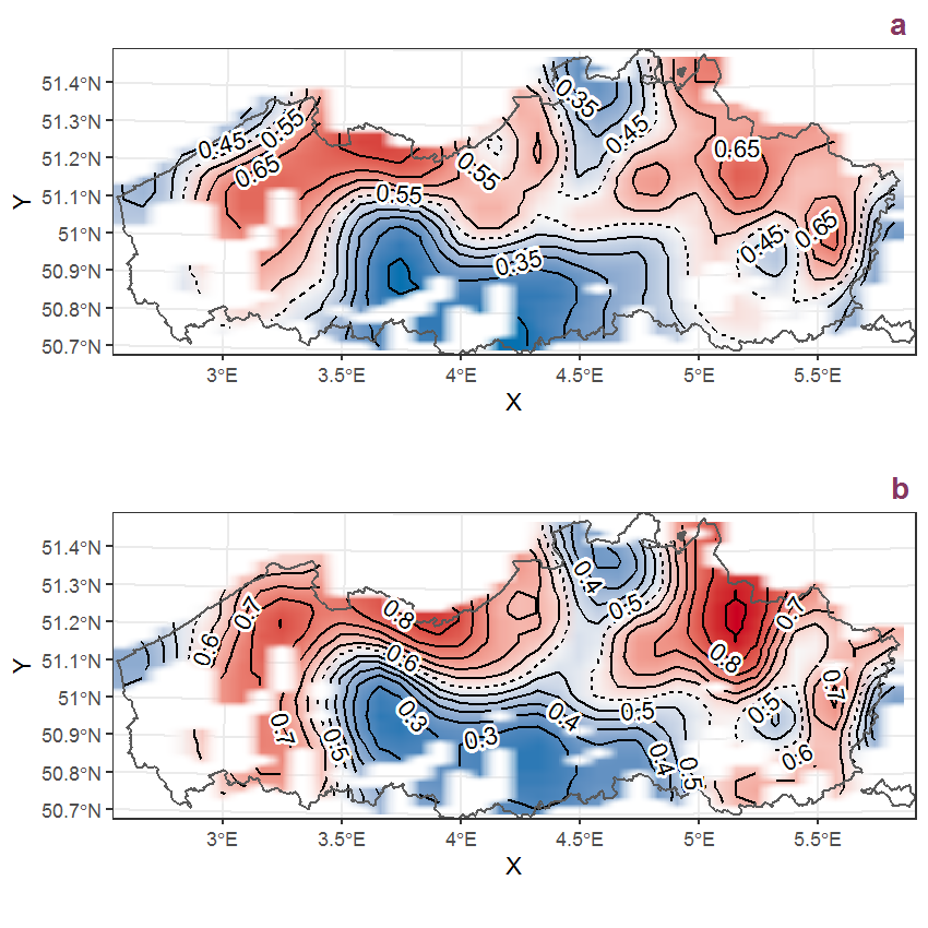
Figure T.50: Visualisation of the spatial smooth effect on the probability of Trifolium arvense L. presence in 1 km x 1 km squares where the species has been observed at least once. The probabilities (values on the contour lines) are conditional on the final year of observation and a list-length equal to 130. The dashed contour line demarcates zones where the species is expected to be more prevalent (red shades) from zones where the species is less prevalent (blue shades). a: 1950 - 2018, b: 1990 - 2018.
T.18 Trifolium campestre Schreb.
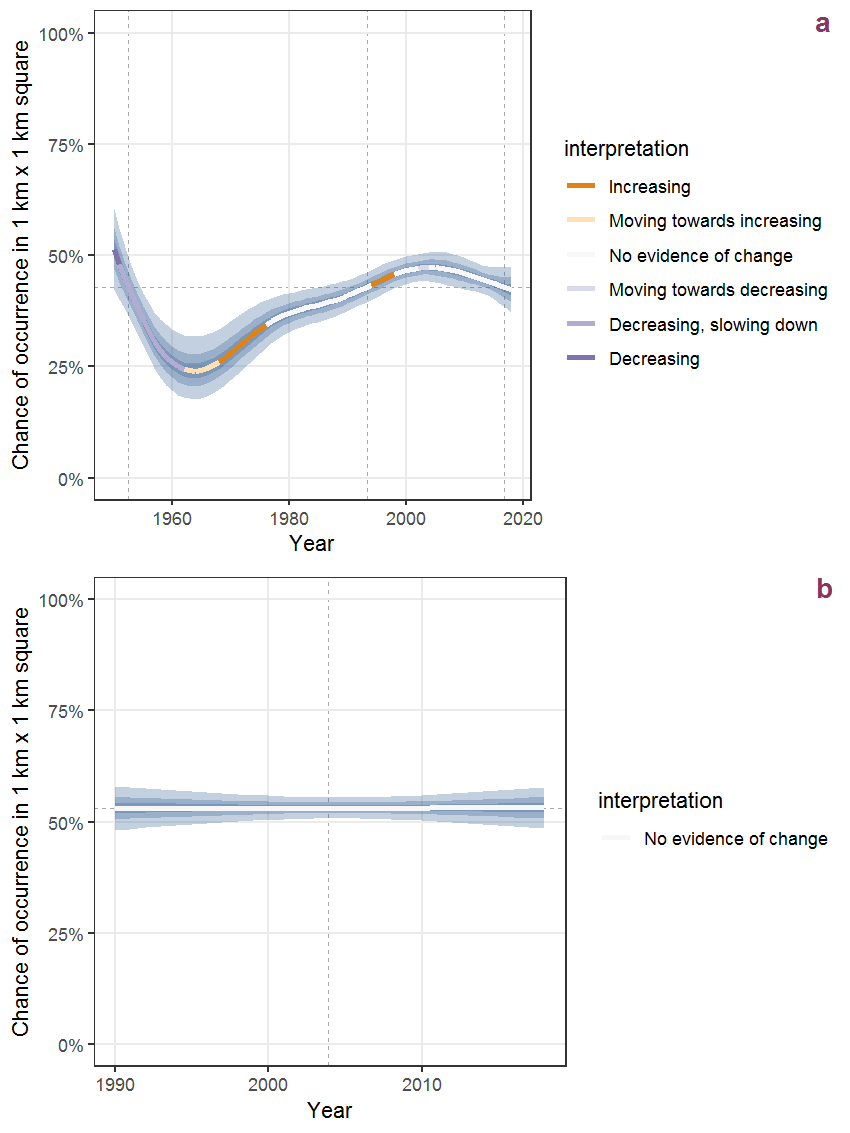
Figure T.51: Effect of year on the probability of Trifolium campestre Schreb. presence in 1 km x 1 km squares where the species has been observed at least once. The fitted line shows the sum of the overall mean (the intercept), a conditional effect of list-length equal to 130 and the year-smoother. The vertical dashed lines indicate the year(s) where the year-smoother is zero. The 95% confidence band is shown in grey (including the variability around the intercept and the smoother). a: 1950 - 2018, b: 1990 - 2018.
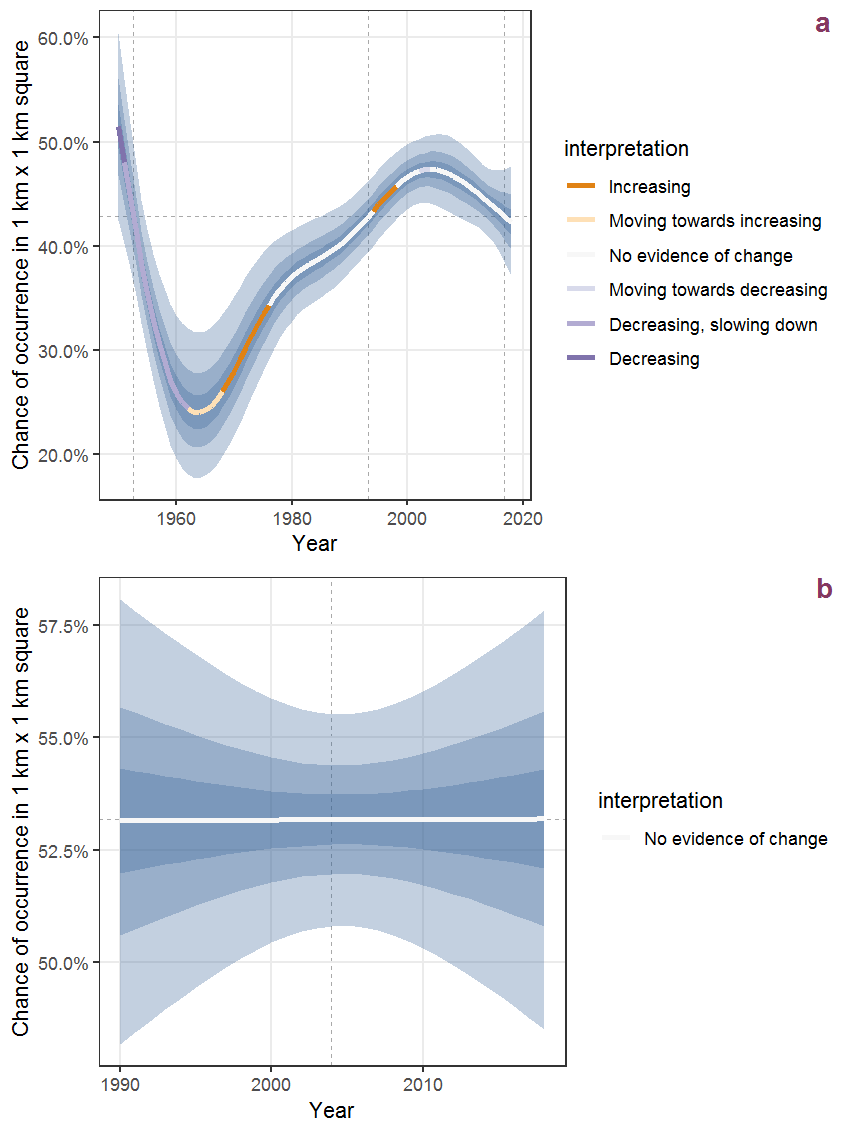
Figure T.52: The same as T.51, but the vertical axis is scaled to the range of the predicted values such that relative changes can be seen more easily. a: 1950 - 2018, b: 1990 - 2018.
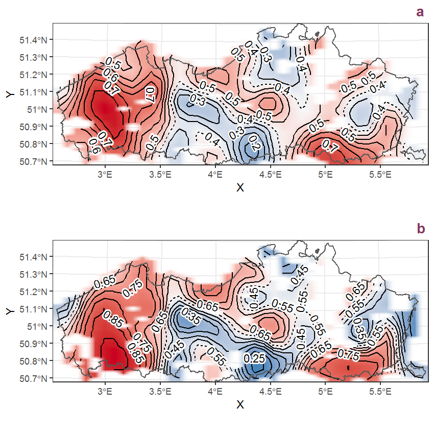
Figure T.53: Visualisation of the spatial smooth effect on the probability of Trifolium campestre Schreb. presence in 1 km x 1 km squares where the species has been observed at least once. The probabilities (values on the contour lines) are conditional on the final year of observation and a list-length equal to 130. The dashed contour line demarcates zones where the species is expected to be more prevalent (red shades) from zones where the species is less prevalent (blue shades). a: 1950 - 2018, b: 1990 - 2018.
T.19 Trifolium dubium Sibth.
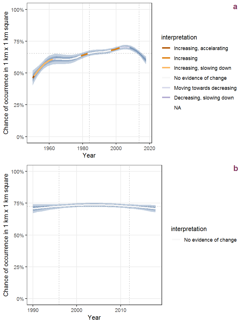
Figure T.54: Effect of year on the probability of Trifolium dubium Sibth. presence in 1 km x 1 km squares where the species has been observed at least once. The fitted line shows the sum of the overall mean (the intercept), a conditional effect of list-length equal to 130 and the year-smoother. The vertical dashed lines indicate the year(s) where the year-smoother is zero. The 95% confidence band is shown in grey (including the variability around the intercept and the smoother). a: 1950 - 2018, b: 1990 - 2018.
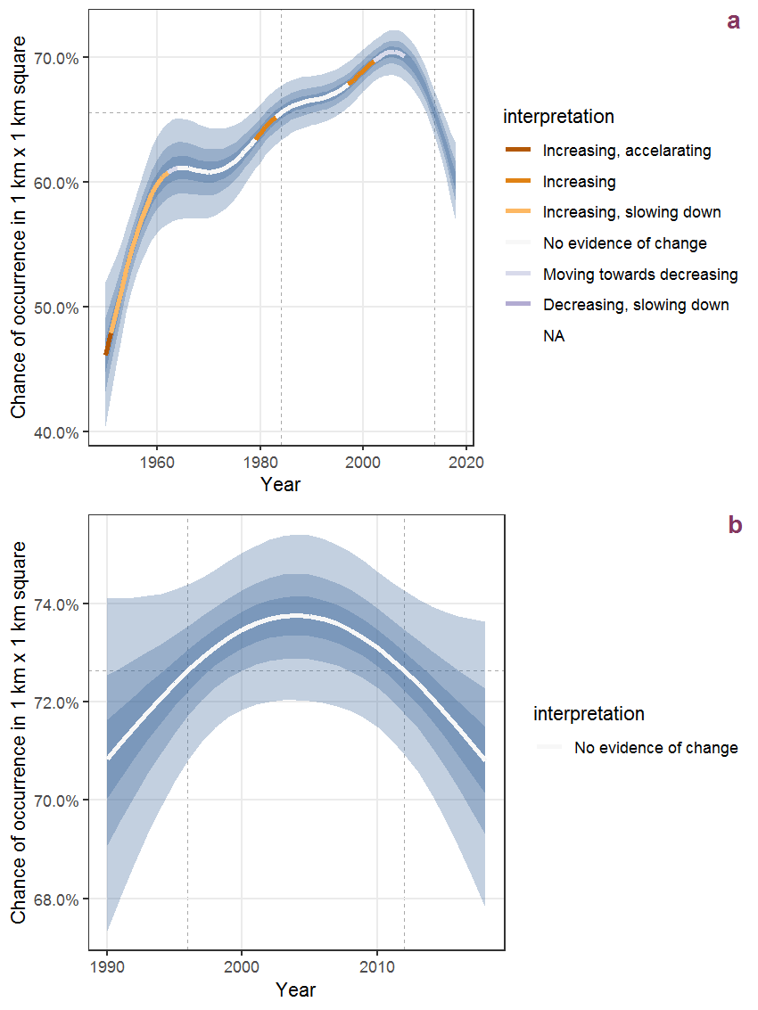
Figure T.55: The same as T.54, but the vertical axis is scaled to the range of the predicted values such that relative changes can be seen more easily. a: 1950 - 2018, b: 1990 - 2018.
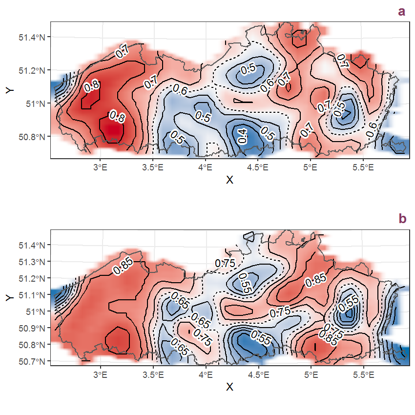
Figure T.56: Visualisation of the spatial smooth effect on the probability of Trifolium dubium Sibth. presence in 1 km x 1 km squares where the species has been observed at least once. The probabilities (values on the contour lines) are conditional on the final year of observation and a list-length equal to 130. The dashed contour line demarcates zones where the species is expected to be more prevalent (red shades) from zones where the species is less prevalent (blue shades). a: 1950 - 2018, b: 1990 - 2018.
T.20 Trifolium fragiferum L.
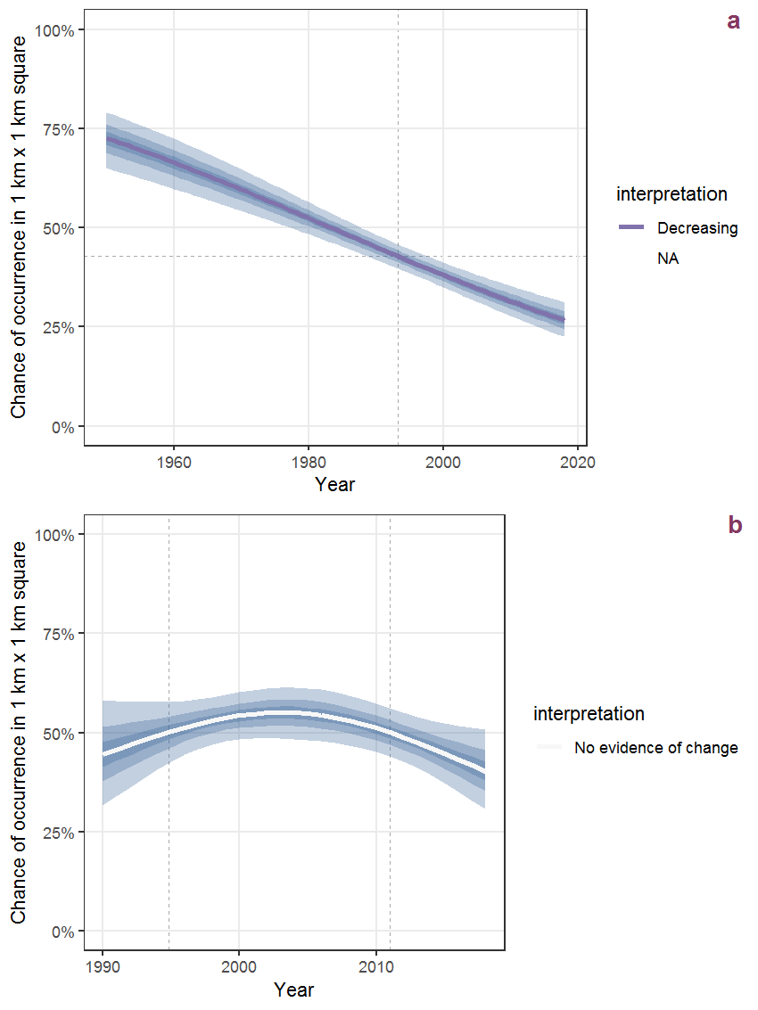
Figure T.57: Effect of year on the probability of Trifolium fragiferum L. presence in 1 km x 1 km squares where the species has been observed at least once. The fitted line shows the sum of the overall mean (the intercept), a conditional effect of list-length equal to 130 and the year-smoother. The vertical dashed lines indicate the year(s) where the year-smoother is zero. The 95% confidence band is shown in grey (including the variability around the intercept and the smoother). a: 1950 - 2018, b: 1990 - 2018.
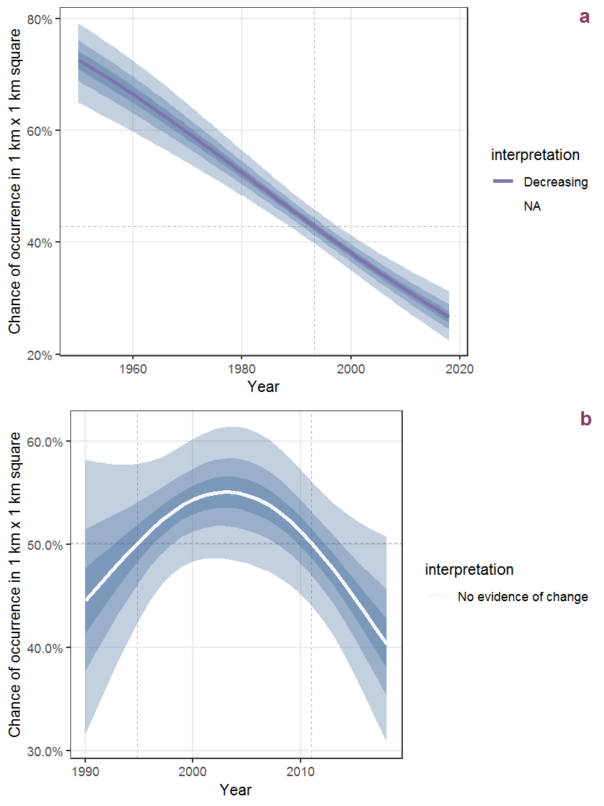
Figure T.58: The same as T.57, but the vertical axis is scaled to the range of the predicted values such that relative changes can be seen more easily. a: 1950 - 2018, b: 1990 - 2018.
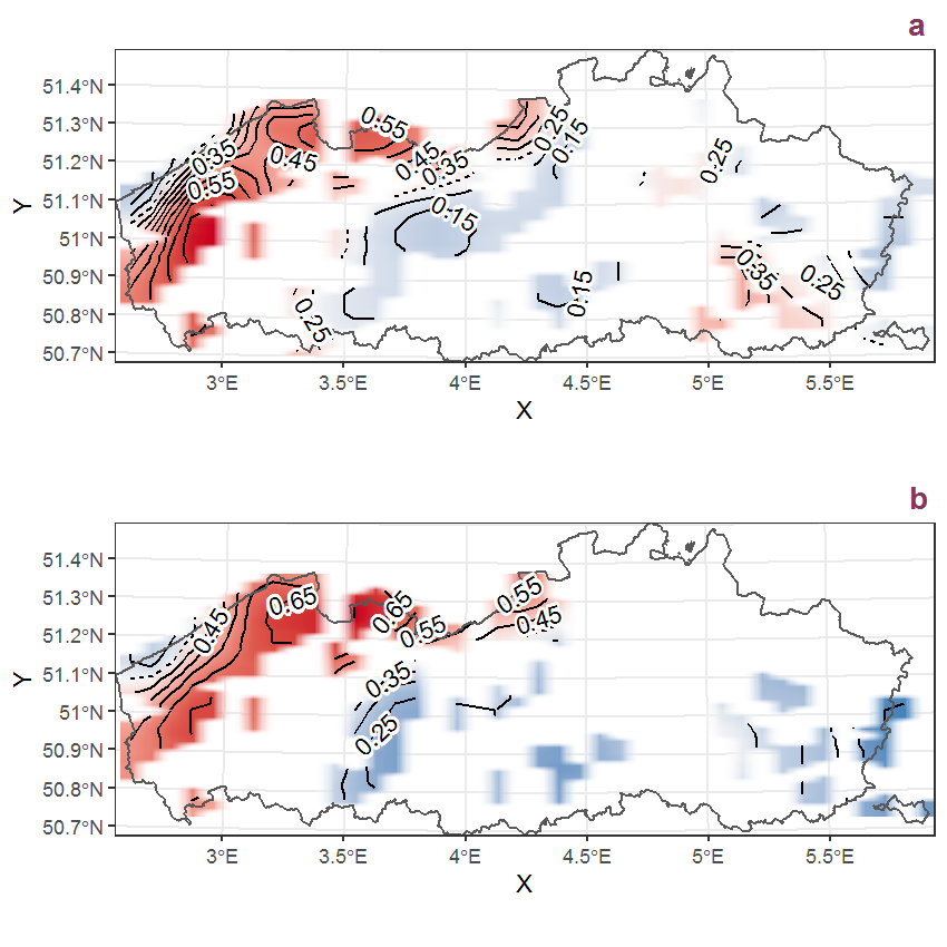
Figure T.59: Visualisation of the spatial smooth effect on the probability of Trifolium fragiferum L. presence in 1 km x 1 km squares where the species has been observed at least once. The probabilities (values on the contour lines) are conditional on the final year of observation and a list-length equal to 130. The dashed contour line demarcates zones where the species is expected to be more prevalent (red shades) from zones where the species is less prevalent (blue shades). a: 1950 - 2018, b: 1990 - 2018.
T.21 Trifolium hybridum L.
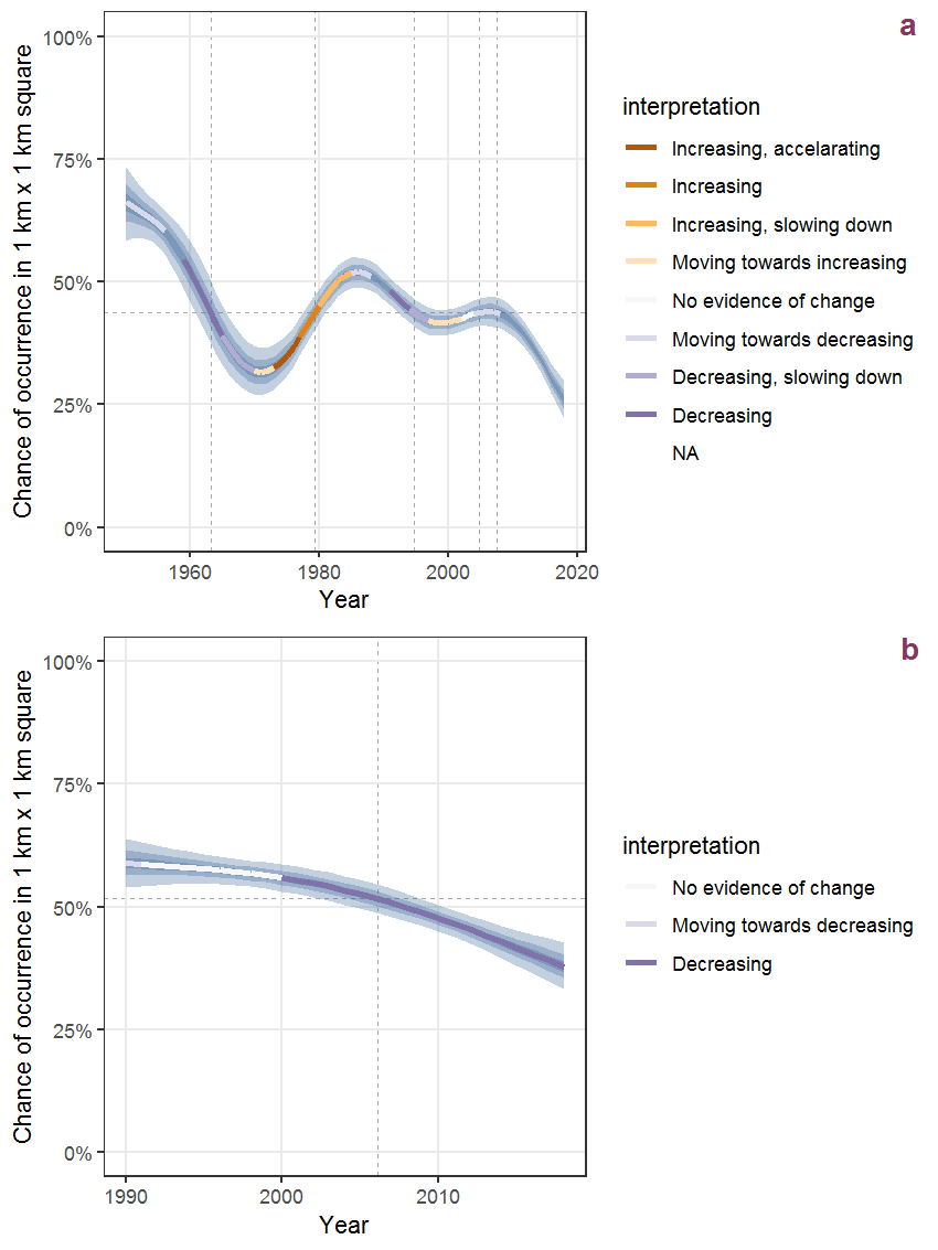
Figure T.60: Effect of year on the probability of Trifolium hybridum L. presence in 1 km x 1 km squares where the species has been observed at least once. The fitted line shows the sum of the overall mean (the intercept), a conditional effect of list-length equal to 130 and the year-smoother. The vertical dashed lines indicate the year(s) where the year-smoother is zero. The 95% confidence band is shown in grey (including the variability around the intercept and the smoother). a: 1950 - 2018, b: 1990 - 2018.
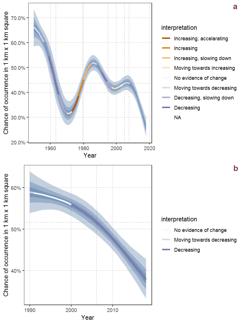
Figure T.61: The same as T.60, but the vertical axis is scaled to the range of the predicted values such that relative changes can be seen more easily. a: 1950 - 2018, b: 1990 - 2018.
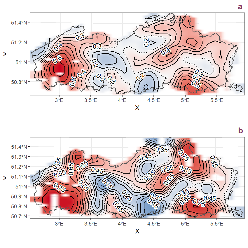
Figure T.62: Visualisation of the spatial smooth effect on the probability of Trifolium hybridum L. presence in 1 km x 1 km squares where the species has been observed at least once. The probabilities (values on the contour lines) are conditional on the final year of observation and a list-length equal to 130. The dashed contour line demarcates zones where the species is expected to be more prevalent (red shades) from zones where the species is less prevalent (blue shades). a: 1950 - 2018, b: 1990 - 2018.
T.22 Trifolium pratense L.
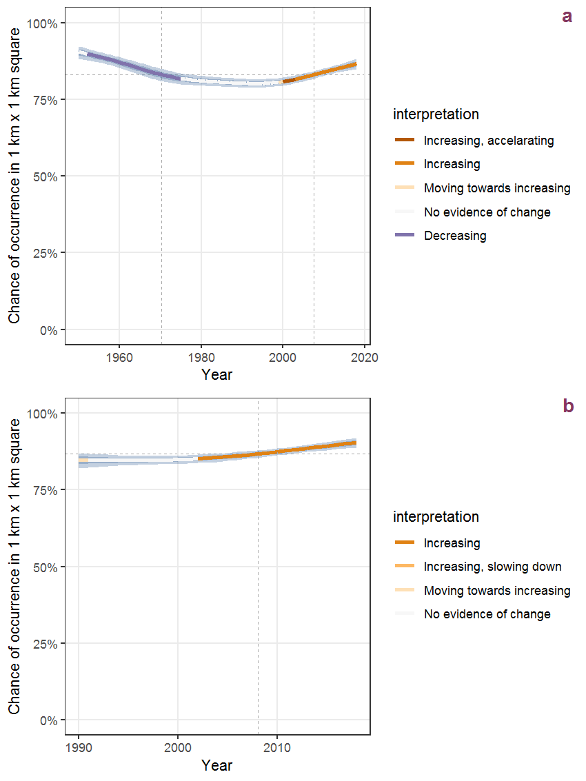
Figure T.63: Effect of year on the probability of Trifolium pratense L. presence in 1 km x 1 km squares where the species has been observed at least once. The fitted line shows the sum of the overall mean (the intercept), a conditional effect of list-length equal to 130 and the year-smoother. The vertical dashed lines indicate the year(s) where the year-smoother is zero. The 95% confidence band is shown in grey (including the variability around the intercept and the smoother). a: 1950 - 2018, b: 1990 - 2018.
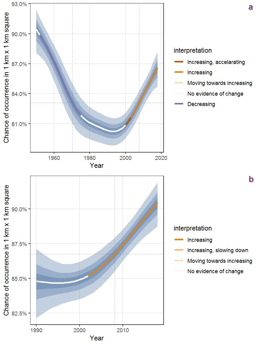
Figure T.64: The same as T.63, but the vertical axis is scaled to the range of the predicted values such that relative changes can be seen more easily. a: 1950 - 2018, b: 1990 - 2018.
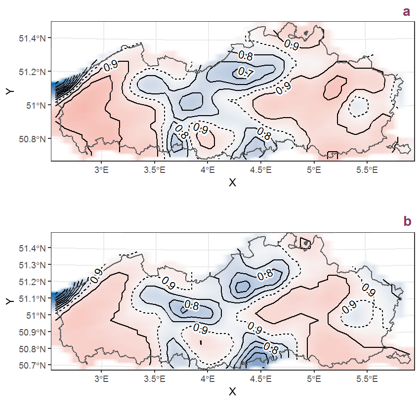
Figure T.65: Visualisation of the spatial smooth effect on the probability of Trifolium pratense L. presence in 1 km x 1 km squares where the species has been observed at least once. The probabilities (values on the contour lines) are conditional on the final year of observation and a list-length equal to 130. The dashed contour line demarcates zones where the species is expected to be more prevalent (red shades) from zones where the species is less prevalent (blue shades). a: 1950 - 2018, b: 1990 - 2018.
T.23 Trifolium repens L.
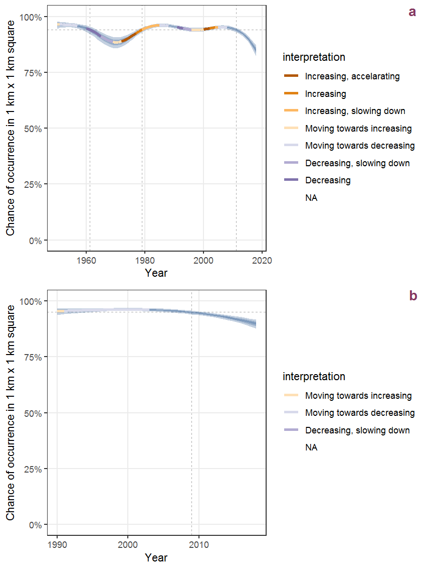
Figure T.66: Effect of year on the probability of Trifolium repens L. presence in 1 km x 1 km squares where the species has been observed at least once. The fitted line shows the sum of the overall mean (the intercept), a conditional effect of list-length equal to 130 and the year-smoother. The vertical dashed lines indicate the year(s) where the year-smoother is zero. The 95% confidence band is shown in grey (including the variability around the intercept and the smoother). a: 1950 - 2018, b: 1990 - 2018.
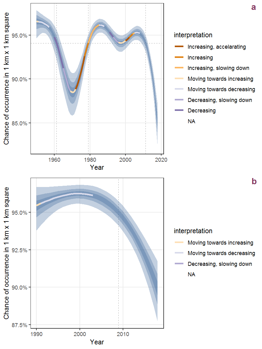
Figure T.67: The same as T.66, but the vertical axis is scaled to the range of the predicted values such that relative changes can be seen more easily. a: 1950 - 2018, b: 1990 - 2018.
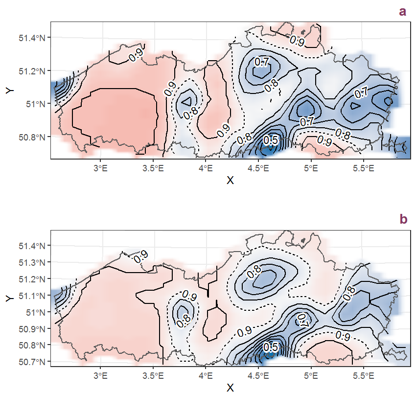
Figure T.68: Visualisation of the spatial smooth effect on the probability of Trifolium repens L. presence in 1 km x 1 km squares where the species has been observed at least once. The probabilities (values on the contour lines) are conditional on the final year of observation and a list-length equal to 130. The dashed contour line demarcates zones where the species is expected to be more prevalent (red shades) from zones where the species is less prevalent (blue shades). a: 1950 - 2018, b: 1990 - 2018.
T.24 Trisetum flavescens (L.) Beauv.
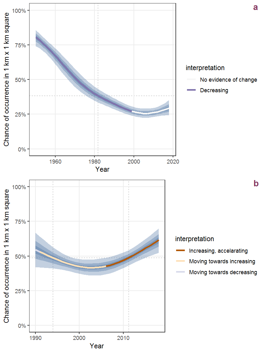
Figure T.69: Effect of year on the probability of Trisetum flavescens (L.) Beauv. presence in 1 km x 1 km squares where the species has been observed at least once. The fitted line shows the sum of the overall mean (the intercept), a conditional effect of list-length equal to 130 and the year-smoother. The vertical dashed lines indicate the year(s) where the year-smoother is zero. The 95% confidence band is shown in grey (including the variability around the intercept and the smoother). a: 1950 - 2018, b: 1990 - 2018.
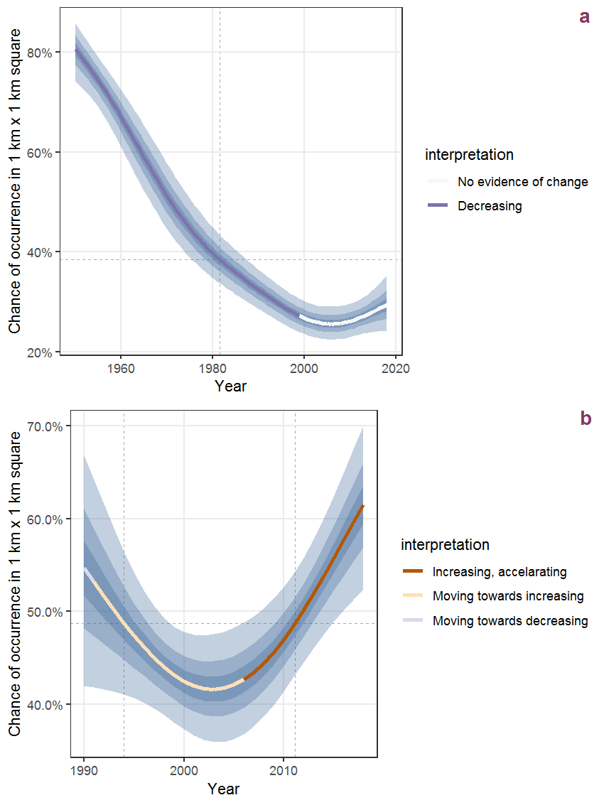
Figure T.70: The same as T.69, but the vertical axis is scaled to the range of the predicted values such that relative changes can be seen more easily. a: 1950 - 2018, b: 1990 - 2018.
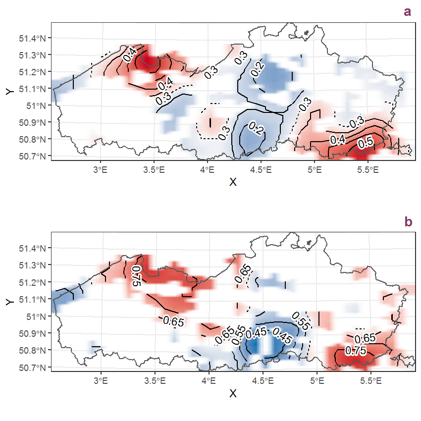
Figure T.71: Visualisation of the spatial smooth effect on the probability of Trisetum flavescens (L.) Beauv. presence in 1 km x 1 km squares where the species has been observed at least once. The probabilities (values on the contour lines) are conditional on the final year of observation and a list-length equal to 130. The dashed contour line demarcates zones where the species is expected to be more prevalent (red shades) from zones where the species is less prevalent (blue shades). a: 1950 - 2018, b: 1990 - 2018.
T.25 Tussilago farfara L.
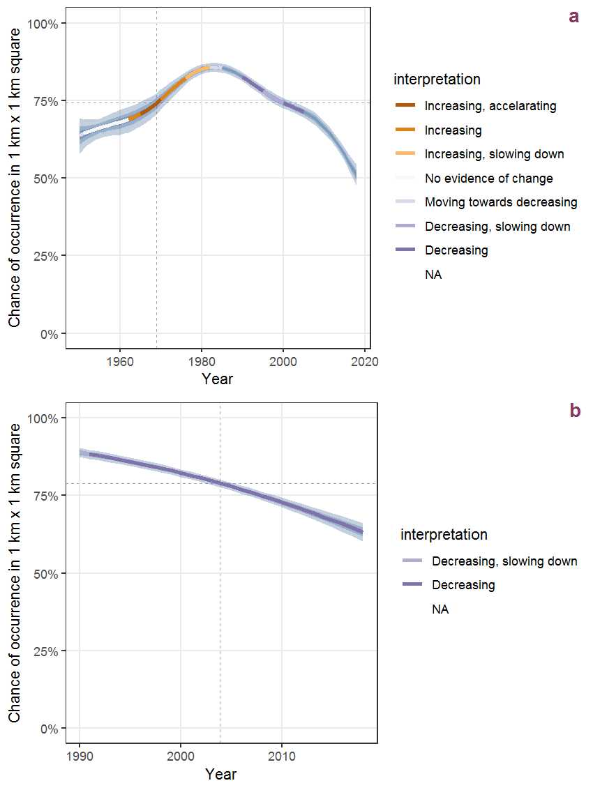
Figure T.72: Effect of year on the probability of Tussilago farfara L. presence in 1 km x 1 km squares where the species has been observed at least once. The fitted line shows the sum of the overall mean (the intercept), a conditional effect of list-length equal to 130 and the year-smoother. The vertical dashed lines indicate the year(s) where the year-smoother is zero. The 95% confidence band is shown in grey (including the variability around the intercept and the smoother). a: 1950 - 2018, b: 1990 - 2018.
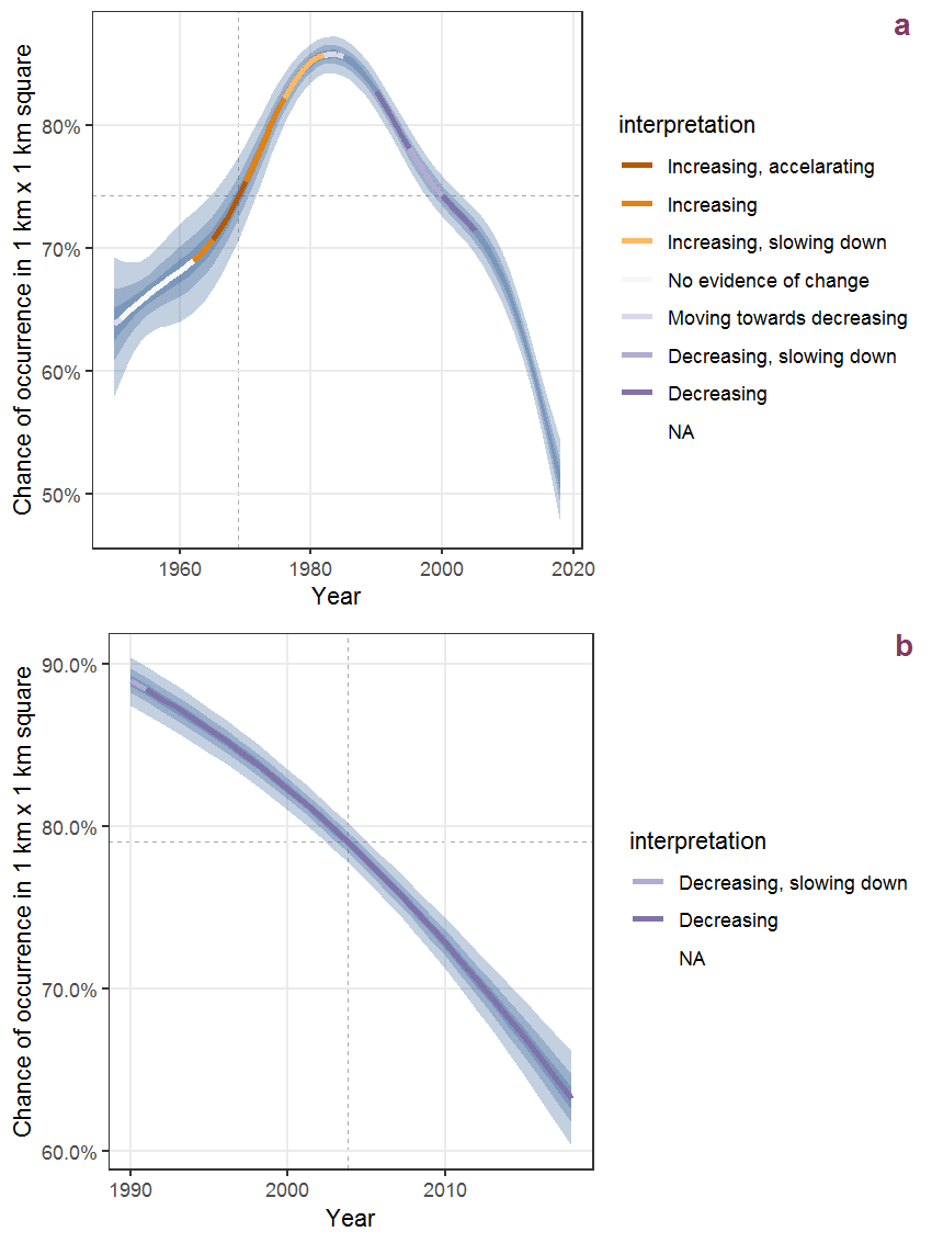
Figure T.73: The same as T.72, but the vertical axis is scaled to the range of the predicted values such that relative changes can be seen more easily. a: 1950 - 2018, b: 1990 - 2018.
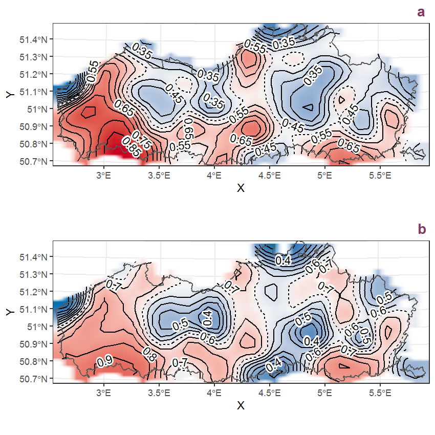
Figure T.74: Visualisation of the spatial smooth effect on the probability of Tussilago farfara L. presence in 1 km x 1 km squares where the species has been observed at least once. The probabilities (values on the contour lines) are conditional on the final year of observation and a list-length equal to 130. The dashed contour line demarcates zones where the species is expected to be more prevalent (red shades) from zones where the species is less prevalent (blue shades). a: 1950 - 2018, b: 1990 - 2018.
T.26 Typha angustifolia L.
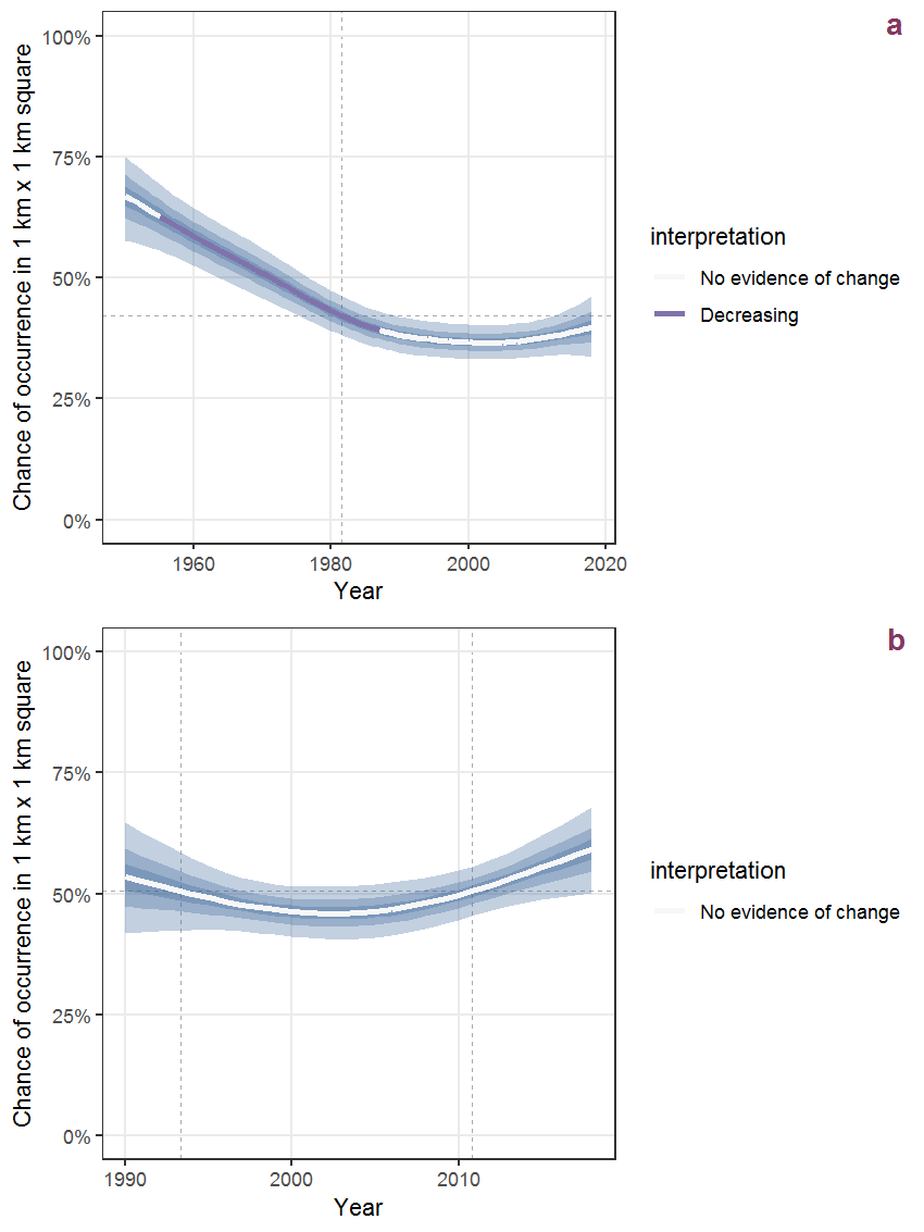
Figure T.75: Effect of year on the probability of Typha angustifolia L. presence in 1 km x 1 km squares where the species has been observed at least once. The fitted line shows the sum of the overall mean (the intercept), a conditional effect of list-length equal to 130 and the year-smoother. The vertical dashed lines indicate the year(s) where the year-smoother is zero. The 95% confidence band is shown in grey (including the variability around the intercept and the smoother). a: 1950 - 2018, b: 1990 - 2018.
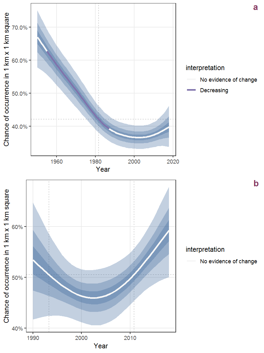
Figure T.76: The same as T.75, but the vertical axis is scaled to the range of the predicted values such that relative changes can be seen more easily. a: 1950 - 2018, b: 1990 - 2018.
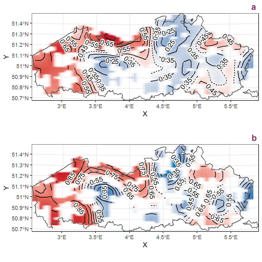
Figure T.77: Visualisation of the spatial smooth effect on the probability of Typha angustifolia L. presence in 1 km x 1 km squares where the species has been observed at least once. The probabilities (values on the contour lines) are conditional on the final year of observation and a list-length equal to 130. The dashed contour line demarcates zones where the species is expected to be more prevalent (red shades) from zones where the species is less prevalent (blue shades). a: 1950 - 2018, b: 1990 - 2018.
T.27 Typha latifolia L.
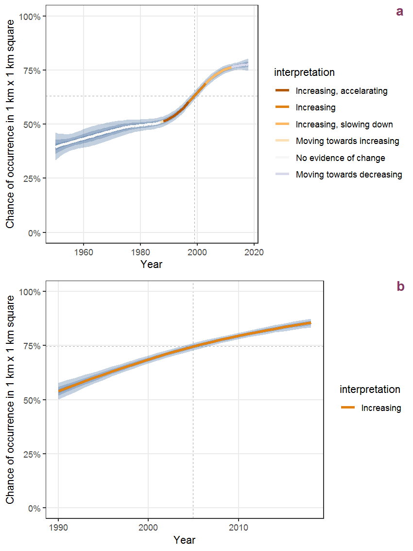
Figure T.78: Effect of year on the probability of Typha latifolia L. presence in 1 km x 1 km squares where the species has been observed at least once. The fitted line shows the sum of the overall mean (the intercept), a conditional effect of list-length equal to 130 and the year-smoother. The vertical dashed lines indicate the year(s) where the year-smoother is zero. The 95% confidence band is shown in grey (including the variability around the intercept and the smoother). a: 1950 - 2018, b: 1990 - 2018.
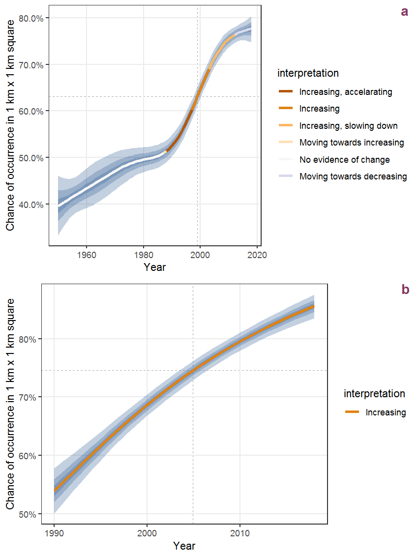
Figure T.79: The same as T.78, but the vertical axis is scaled to the range of the predicted values such that relative changes can be seen more easily. a: 1950 - 2018, b: 1990 - 2018.
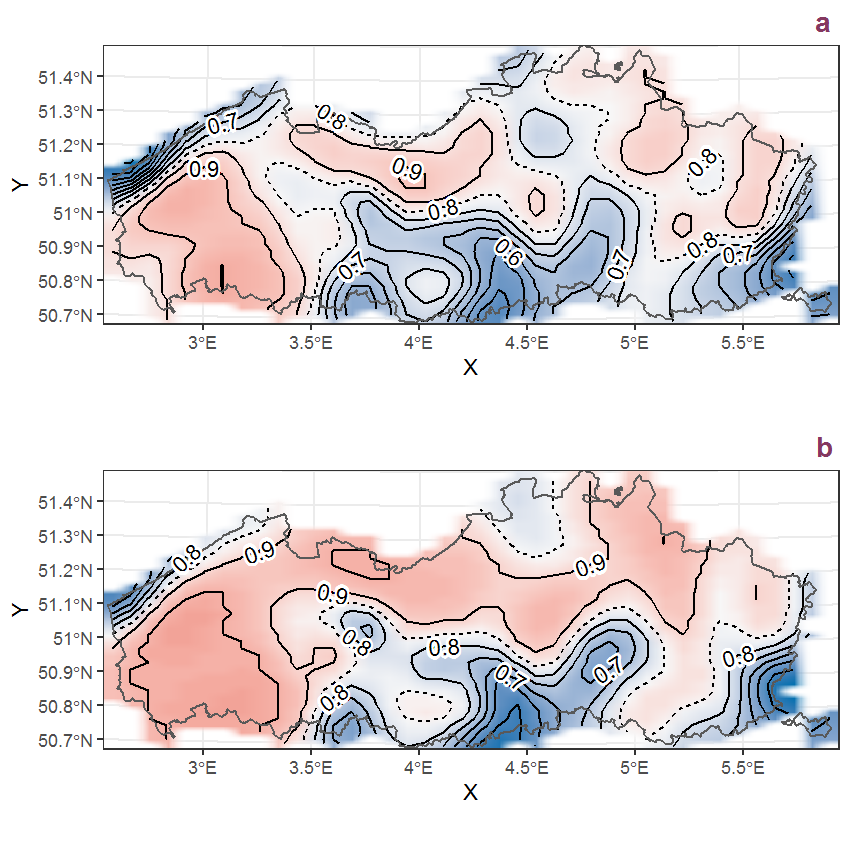
Figure T.80: Visualisation of the spatial smooth effect on the probability of Typha latifolia L. presence in 1 km x 1 km squares where the species has been observed at least once. The probabilities (values on the contour lines) are conditional on the final year of observation and a list-length equal to 130. The dashed contour line demarcates zones where the species is expected to be more prevalent (red shades) from zones where the species is less prevalent (blue shades). a: 1950 - 2018, b: 1990 - 2018.
T.28 Ulmus glabra Huds.
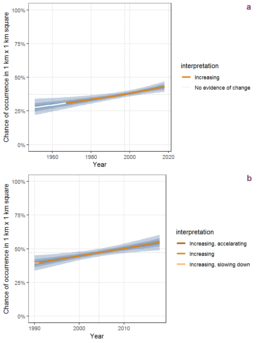
Figure T.81: Effect of year on the probability of Ulmus glabra Huds. presence in 1 km x 1 km squares where the species has been observed at least once. The fitted line shows the sum of the overall mean (the intercept), a conditional effect of list-length equal to 130 and the year-smoother. The vertical dashed lines indicate the year(s) where the year-smoother is zero. The 95% confidence band is shown in grey (including the variability around the intercept and the smoother). a: 1950 - 2018, b: 1990 - 2018.
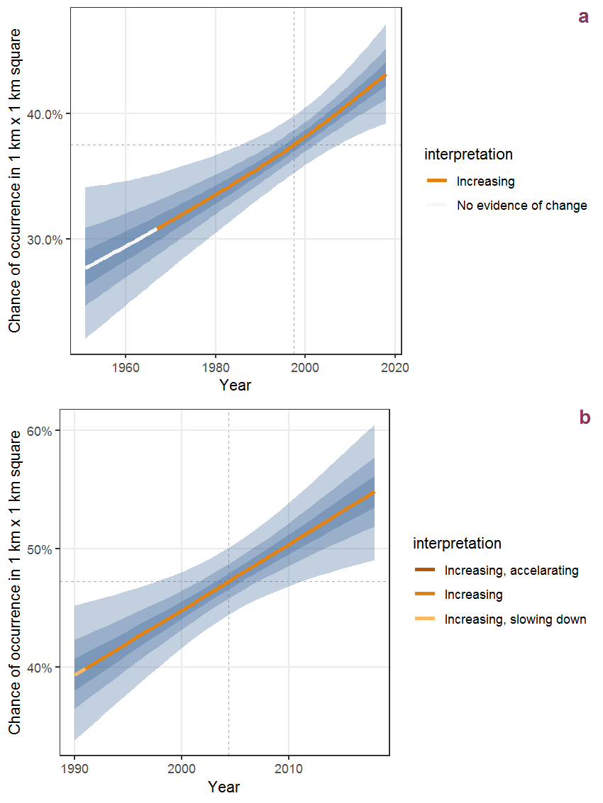
Figure T.82: The same as T.81, but the vertical axis is scaled to the range of the predicted values such that relative changes can be seen more easily. a: 1950 - 2018, b: 1990 - 2018.
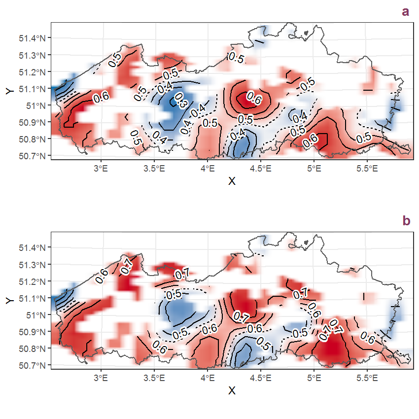
Figure T.83: Visualisation of the spatial smooth effect on the probability of Ulmus glabra Huds. presence in 1 km x 1 km squares where the species has been observed at least once. The probabilities (values on the contour lines) are conditional on the final year of observation and a list-length equal to 130. The dashed contour line demarcates zones where the species is expected to be more prevalent (red shades) from zones where the species is less prevalent (blue shades). a: 1950 - 2018, b: 1990 - 2018.
T.29 Ulmus minor Mill.
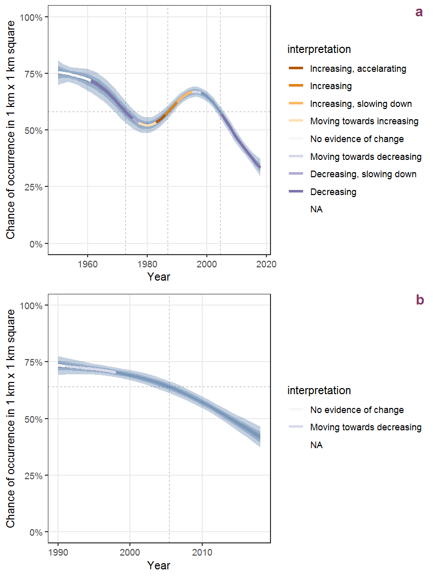
Figure T.84: Effect of year on the probability of Ulmus minor Mill. presence in 1 km x 1 km squares where the species has been observed at least once. The fitted line shows the sum of the overall mean (the intercept), a conditional effect of list-length equal to 130 and the year-smoother. The vertical dashed lines indicate the year(s) where the year-smoother is zero. The 95% confidence band is shown in grey (including the variability around the intercept and the smoother). a: 1950 - 2018, b: 1990 - 2018.
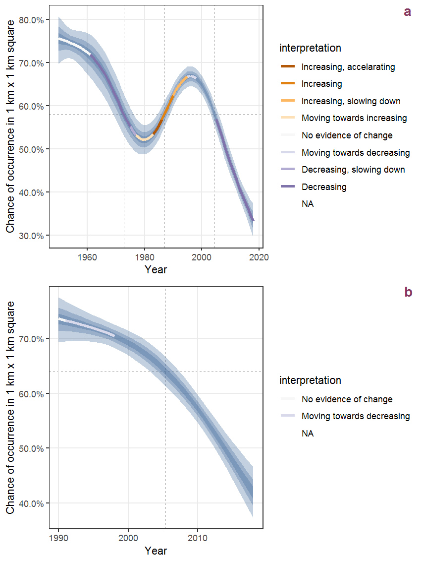
Figure T.85: The same as T.84, but the vertical axis is scaled to the range of the predicted values such that relative changes can be seen more easily. a: 1950 - 2018, b: 1990 - 2018.
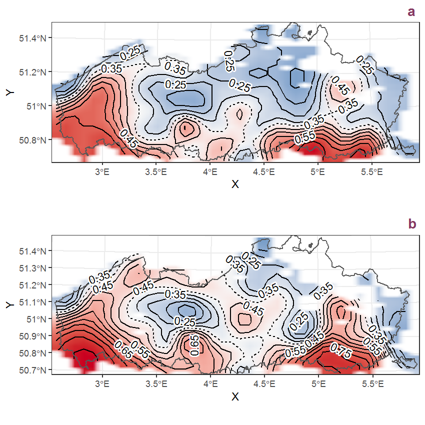
Figure T.86: Visualisation of the spatial smooth effect on the probability of Ulmus minor Mill. presence in 1 km x 1 km squares where the species has been observed at least once. The probabilities (values on the contour lines) are conditional on the final year of observation and a list-length equal to 130. The dashed contour line demarcates zones where the species is expected to be more prevalent (red shades) from zones where the species is less prevalent (blue shades). a: 1950 - 2018, b: 1990 - 2018.
T.30 Urtica dioica L.
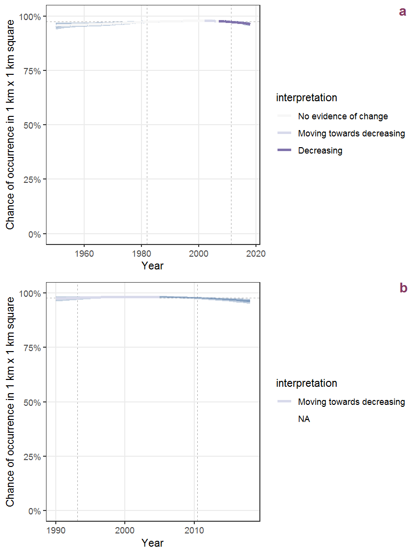
Figure T.87: Effect of year on the probability of Urtica dioica L. presence in 1 km x 1 km squares where the species has been observed at least once. The fitted line shows the sum of the overall mean (the intercept), a conditional effect of list-length equal to 130 and the year-smoother. The vertical dashed lines indicate the year(s) where the year-smoother is zero. The 95% confidence band is shown in grey (including the variability around the intercept and the smoother). a: 1950 - 2018, b: 1990 - 2018.
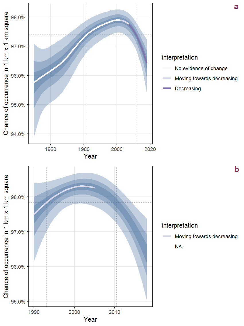
Figure T.88: The same as T.87, but the vertical axis is scaled to the range of the predicted values such that relative changes can be seen more easily. a: 1950 - 2018, b: 1990 - 2018.
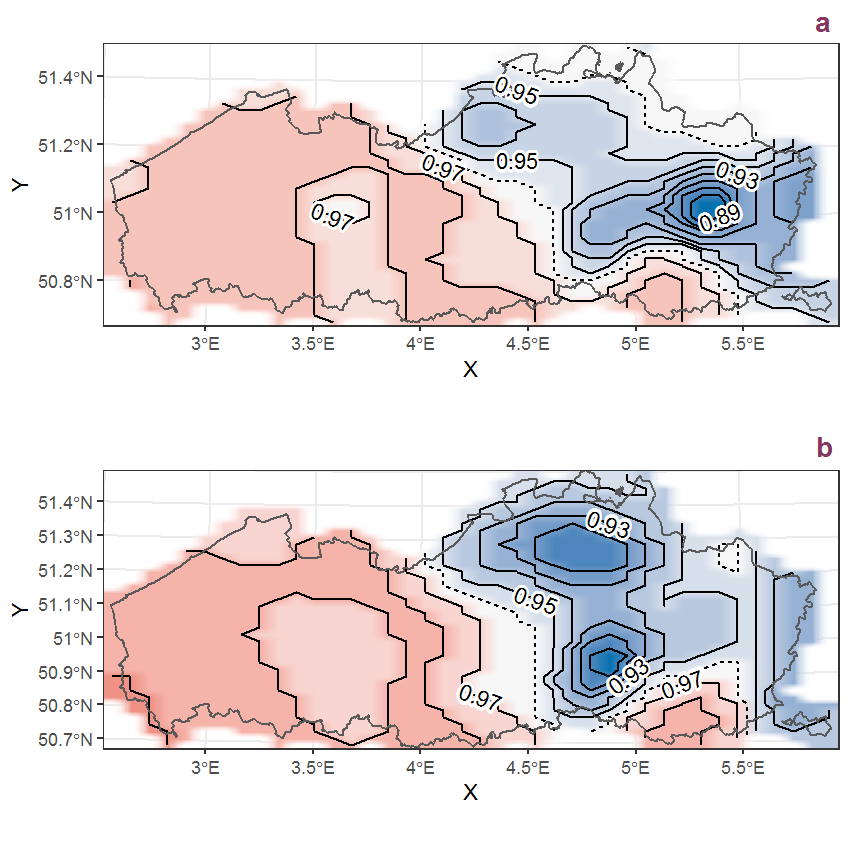
Figure T.89: Visualisation of the spatial smooth effect on the probability of Urtica dioica L. presence in 1 km x 1 km squares where the species has been observed at least once. The probabilities (values on the contour lines) are conditional on the final year of observation and a list-length equal to 130. The dashed contour line demarcates zones where the species is expected to be more prevalent (red shades) from zones where the species is less prevalent (blue shades). a: 1950 - 2018, b: 1990 - 2018.
T.31 Urtica urens L.
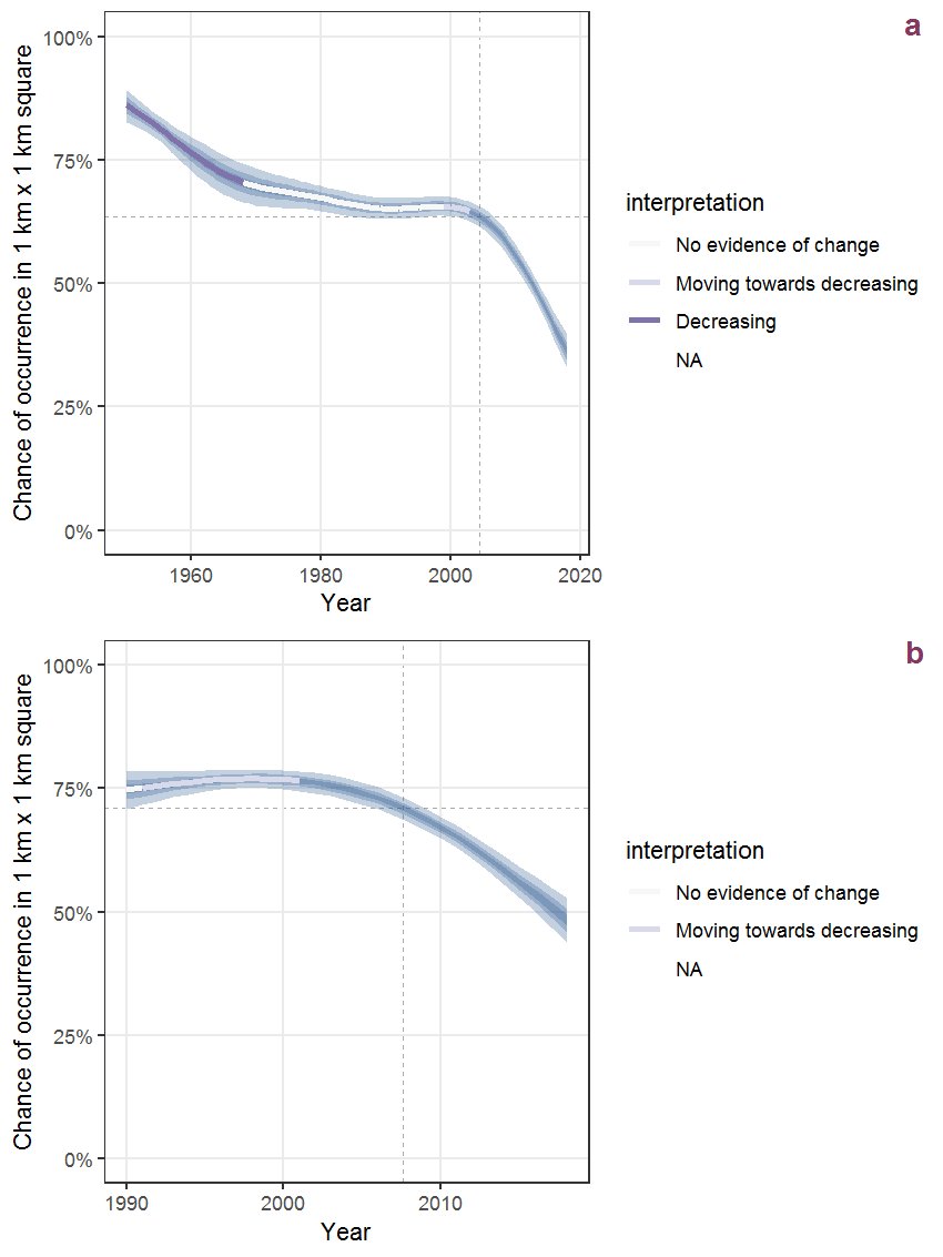
Figure T.90: Effect of year on the probability of Urtica urens L. presence in 1 km x 1 km squares where the species has been observed at least once. The fitted line shows the sum of the overall mean (the intercept), a conditional effect of list-length equal to 130 and the year-smoother. The vertical dashed lines indicate the year(s) where the year-smoother is zero. The 95% confidence band is shown in grey (including the variability around the intercept and the smoother). a: 1950 - 2018, b: 1990 - 2018.
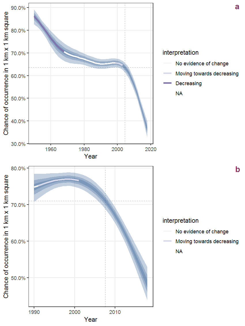
Figure T.91: The same as T.90, but the vertical axis is scaled to the range of the predicted values such that relative changes can be seen more easily. a: 1950 - 2018, b: 1990 - 2018.
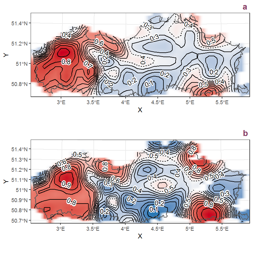
Figure T.92: Visualisation of the spatial smooth effect on the probability of Urtica urens L. presence in 1 km x 1 km squares where the species has been observed at least once. The probabilities (values on the contour lines) are conditional on the final year of observation and a list-length equal to 130. The dashed contour line demarcates zones where the species is expected to be more prevalent (red shades) from zones where the species is less prevalent (blue shades). a: 1950 - 2018, b: 1990 - 2018.
T.32 Vaccinium myrtillus L.
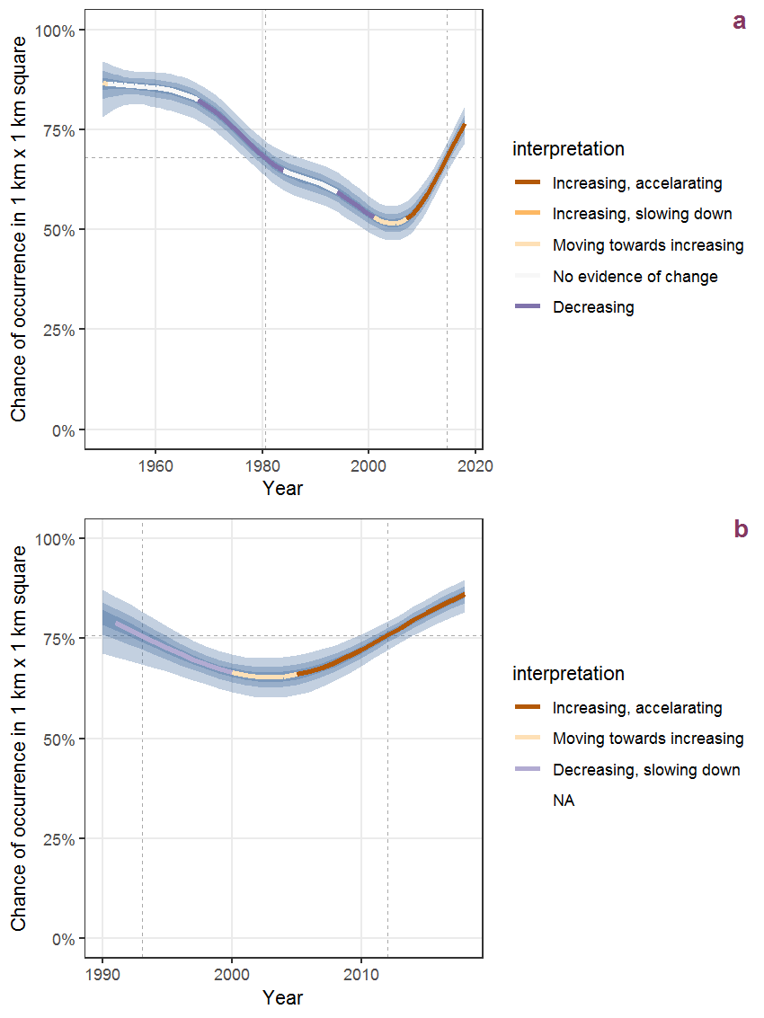
Figure T.93: Effect of year on the probability of Vaccinium myrtillus L. presence in 1 km x 1 km squares where the species has been observed at least once. The fitted line shows the sum of the overall mean (the intercept), a conditional effect of list-length equal to 130 and the year-smoother. The vertical dashed lines indicate the year(s) where the year-smoother is zero. The 95% confidence band is shown in grey (including the variability around the intercept and the smoother). a: 1950 - 2018, b: 1990 - 2018.
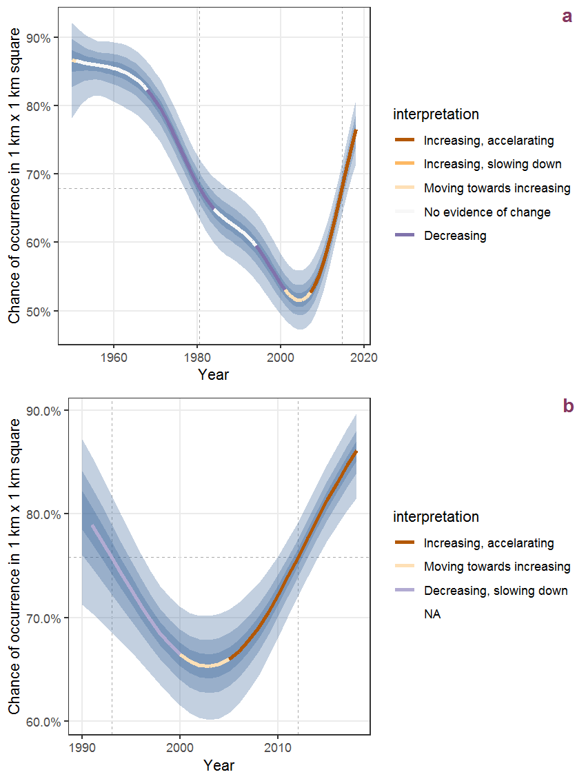
Figure T.94: The same as T.93, but the vertical axis is scaled to the range of the predicted values such that relative changes can be seen more easily. a: 1950 - 2018, b: 1990 - 2018.
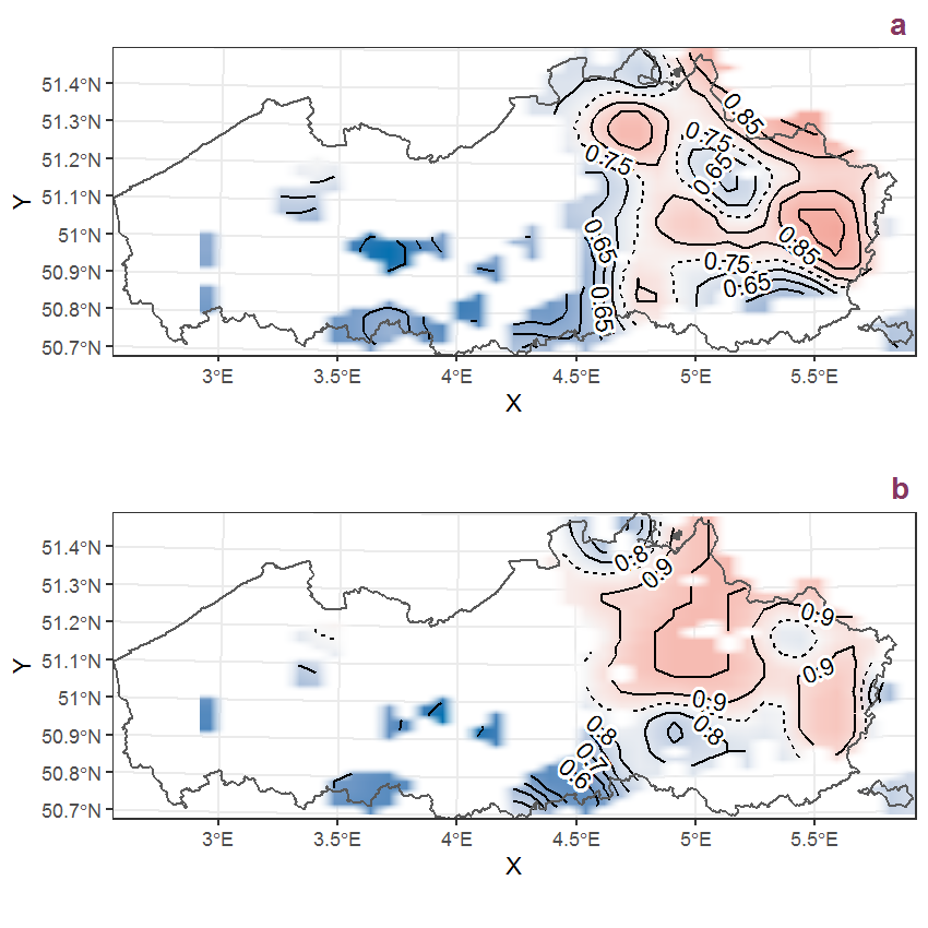
Figure T.95: Visualisation of the spatial smooth effect on the probability of Vaccinium myrtillus L. presence in 1 km x 1 km squares where the species has been observed at least once. The probabilities (values on the contour lines) are conditional on the final year of observation and a list-length equal to 130. The dashed contour line demarcates zones where the species is expected to be more prevalent (red shades) from zones where the species is less prevalent (blue shades). a: 1950 - 2018, b: 1990 - 2018.