F Castanea sativa Mill. - Convallaria majalis L.
F.1 Castanea sativa Mill.
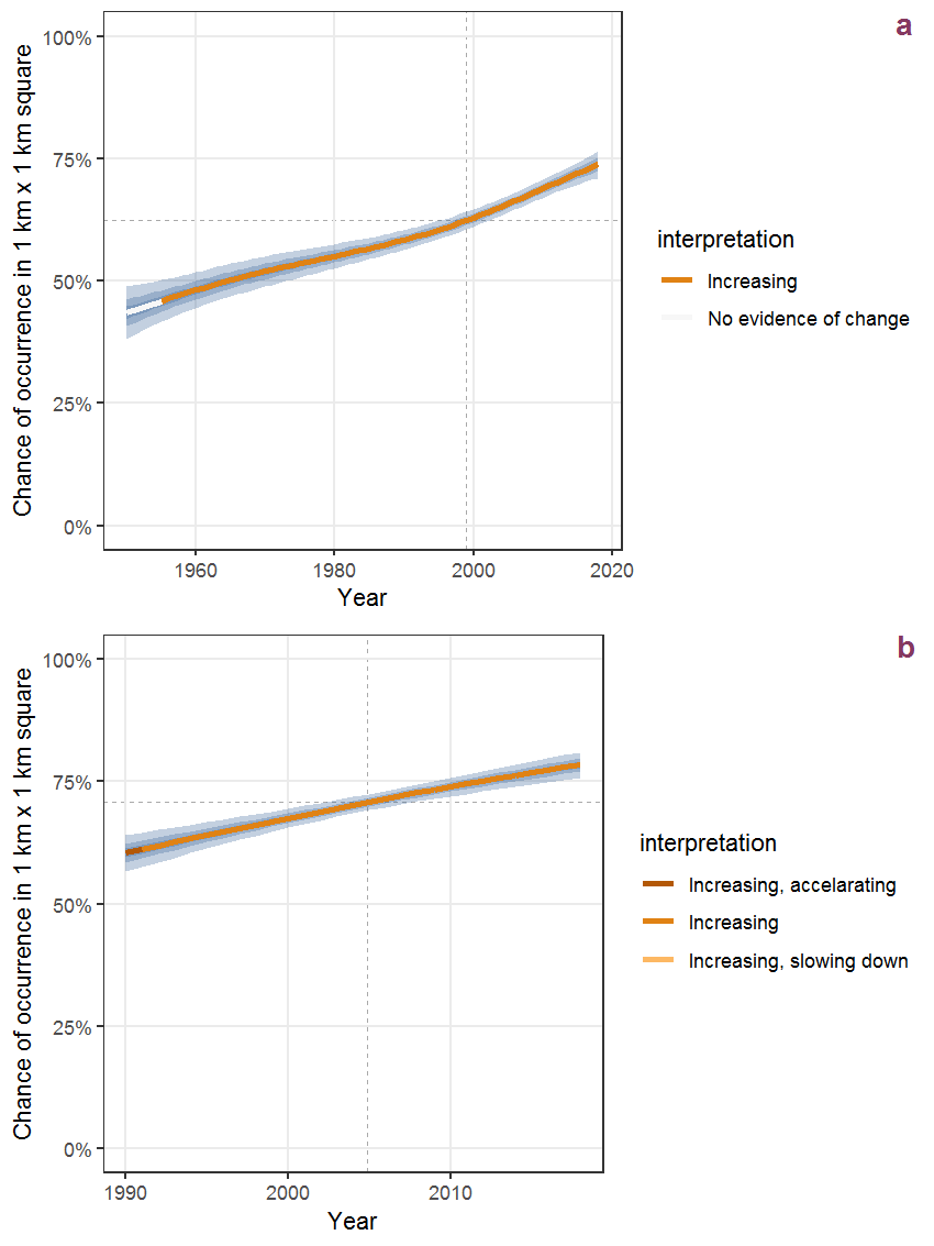
Figure F.1: Effect of year on the probability of Castanea sativa Mill. presence in 1 km x 1 km squares where the species has been observed at least once. The fitted line shows the sum of the overall mean (the intercept), a conditional effect of list-length equal to 130 and the year-smoother. The vertical dashed lines indicate the year(s) where the year-smoother is zero. The 95% confidence band is shown in grey (including the variability around the intercept and the smoother). a: 1950 - 2018, b: 1990 - 2018.
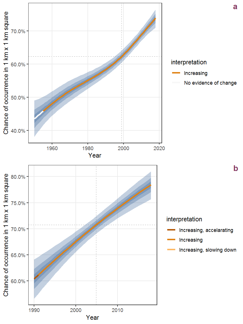
Figure F.2: The same as F.1, but the vertical axis is scaled to the range of the predicted values such that relative changes can be seen more easily. a: 1950 - 2018, b: 1990 - 2018.
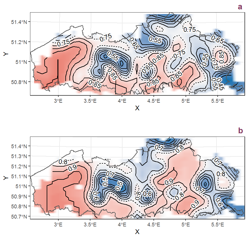
Figure F.3: Visualisation of the spatial smooth effect on the probability of Castanea sativa Mill. presence in 1 km x 1 km squares where the species has been observed at least once. The probabilities (values on the contour lines) are conditional on the final year of observation and a list-length equal to 130. The dashed contour line demarcates zones where the species is expected to be more prevalent (red shades) from zones where the species is less prevalent (blue shades). a: 1950 - 2018, b: 1990 - 2018.
F.2 Centaurea cyanus L.
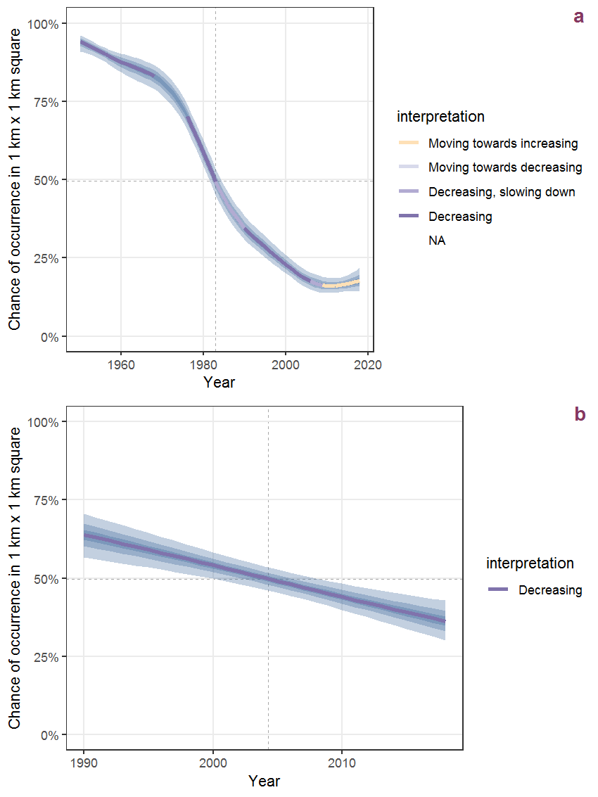
Figure F.4: Effect of year on the probability of Centaurea cyanus L. presence in 1 km x 1 km squares where the species has been observed at least once. The fitted line shows the sum of the overall mean (the intercept), a conditional effect of list-length equal to 130 and the year-smoother. The vertical dashed lines indicate the year(s) where the year-smoother is zero. The 95% confidence band is shown in grey (including the variability around the intercept and the smoother). a: 1950 - 2018, b: 1990 - 2018.
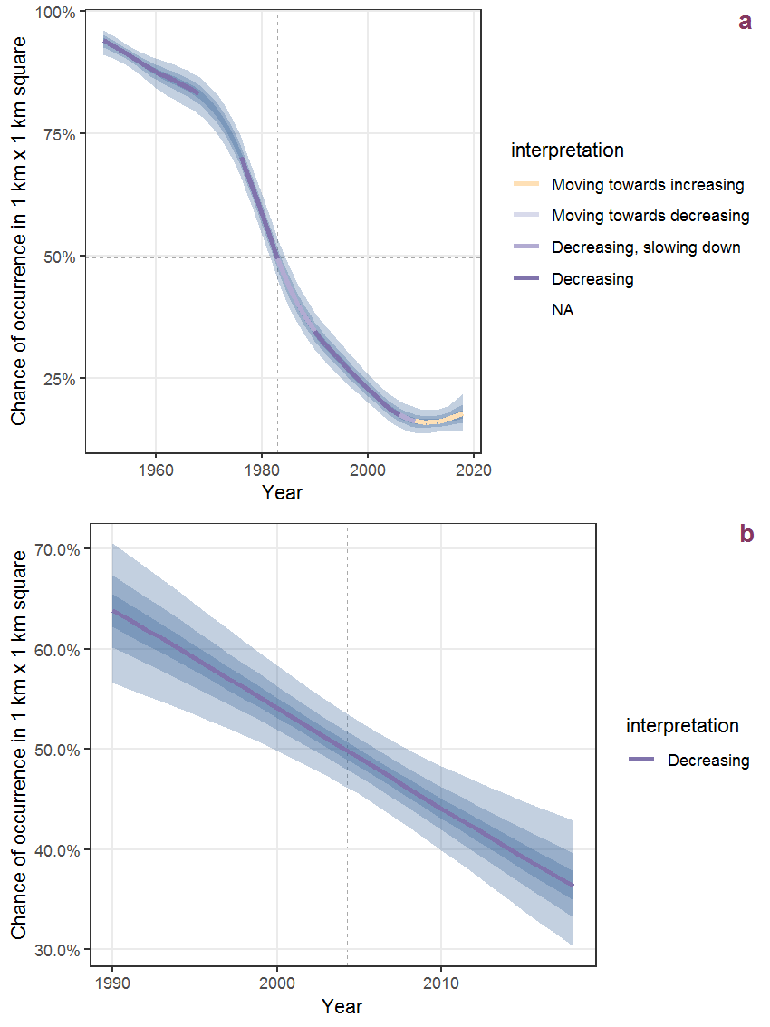
Figure F.5: The same as F.4, but the vertical axis is scaled to the range of the predicted values such that relative changes can be seen more easily. a: 1950 - 2018, b: 1990 - 2018.
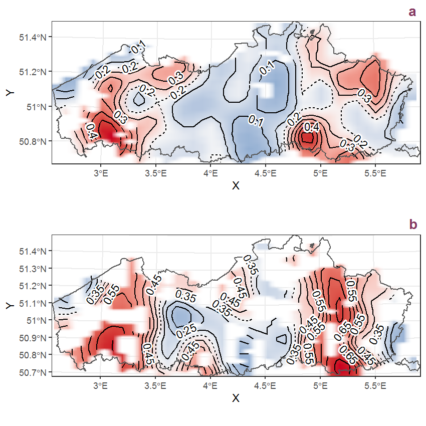
Figure F.6: Visualisation of the spatial smooth effect on the probability of Centaurea cyanus L. presence in 1 km x 1 km squares where the species has been observed at least once. The probabilities (values on the contour lines) are conditional on the final year of observation and a list-length equal to 130. The dashed contour line demarcates zones where the species is expected to be more prevalent (red shades) from zones where the species is less prevalent (blue shades). a: 1950 - 2018, b: 1990 - 2018.
F.3 Centaurea L. subg. Jacea
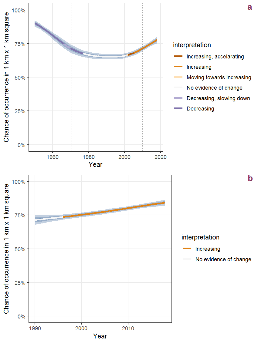
Figure F.7: Effect of year on the probability of Centaurea L. subg. Jacea presence in 1 km x 1 km squares where the species has been observed at least once. The fitted line shows the sum of the overall mean (the intercept), a conditional effect of list-length equal to 130 and the year-smoother. The vertical dashed lines indicate the year(s) where the year-smoother is zero. The 95% confidence band is shown in grey (including the variability around the intercept and the smoother). a: 1950 - 2018, b: 1990 - 2018.
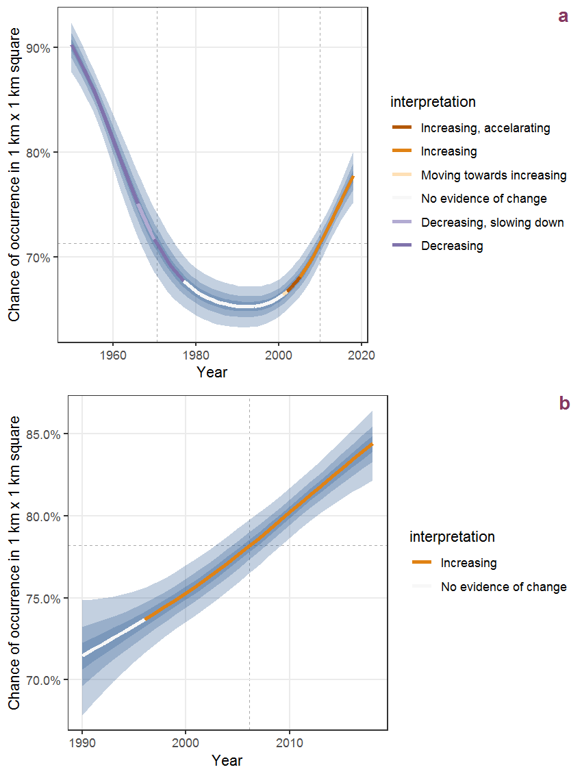
Figure F.8: The same as F.7, but the vertical axis is scaled to the range of the predicted values such that relative changes can be seen more easily. a: 1950 - 2018, b: 1990 - 2018.
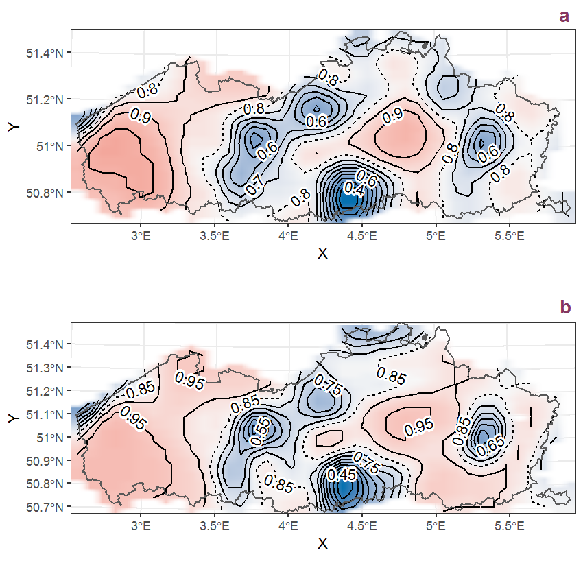
Figure F.9: Visualisation of the spatial smooth effect on the probability of Centaurea L. subg. Jacea presence in 1 km x 1 km squares where the species has been observed at least once. The probabilities (values on the contour lines) are conditional on the final year of observation and a list-length equal to 130. The dashed contour line demarcates zones where the species is expected to be more prevalent (red shades) from zones where the species is less prevalent (blue shades). a: 1950 - 2018, b: 1990 - 2018.
F.4 Centaurium erythraea Rafn
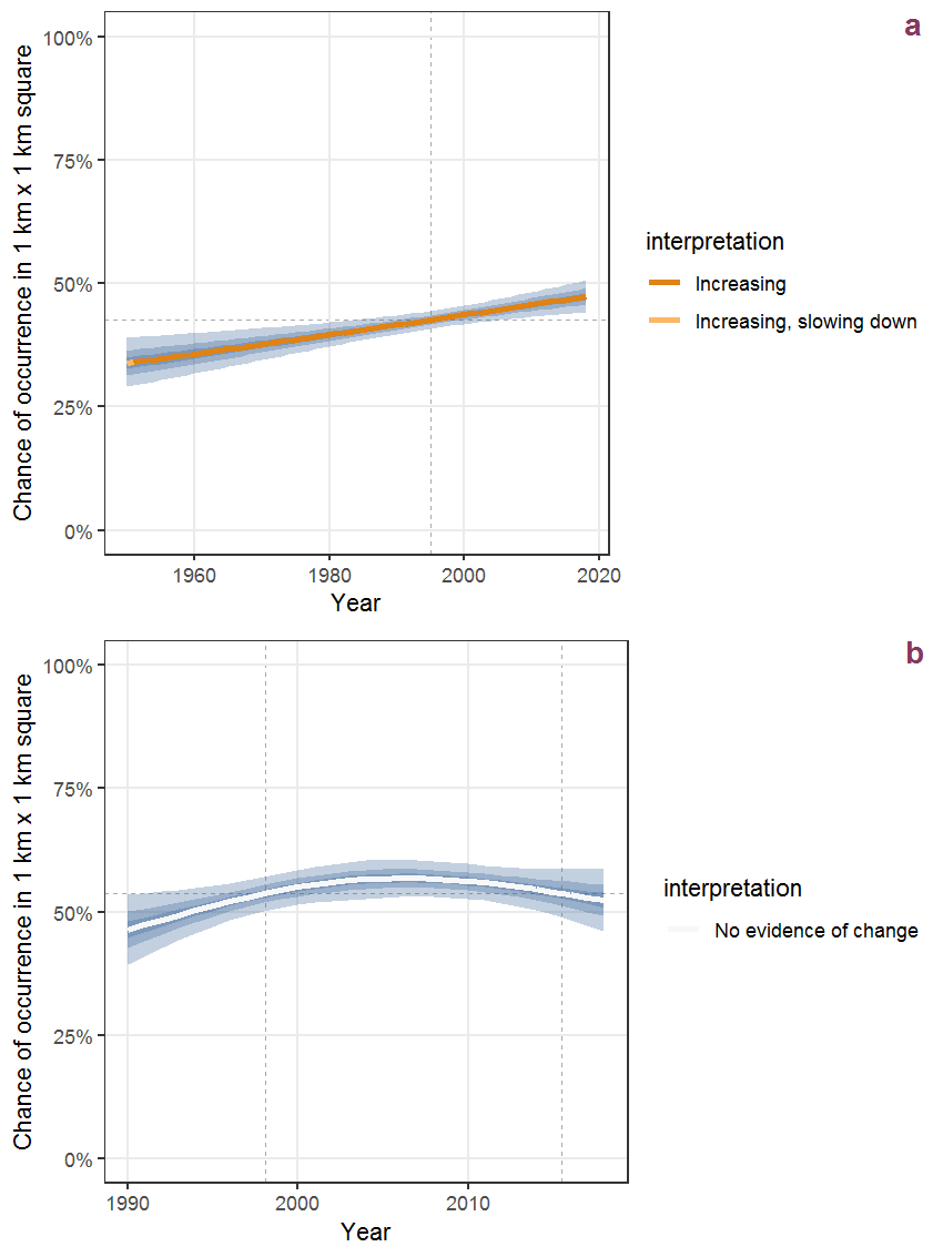
Figure F.10: Effect of year on the probability of Centaurium erythraea Rafn presence in 1 km x 1 km squares where the species has been observed at least once. The fitted line shows the sum of the overall mean (the intercept), a conditional effect of list-length equal to 130 and the year-smoother. The vertical dashed lines indicate the year(s) where the year-smoother is zero. The 95% confidence band is shown in grey (including the variability around the intercept and the smoother). a: 1950 - 2018, b: 1990 - 2018.
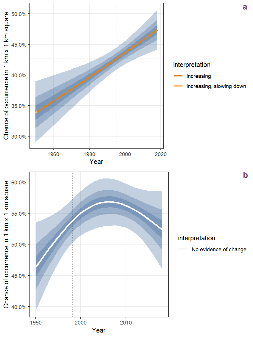
Figure F.11: The same as F.10, but the vertical axis is scaled to the range of the predicted values such that relative changes can be seen more easily. a: 1950 - 2018, b: 1990 - 2018.
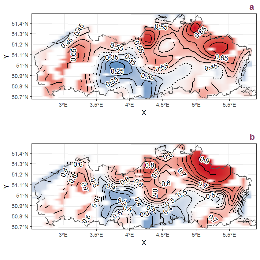
Figure F.12: Visualisation of the spatial smooth effect on the probability of Centaurium erythraea Rafn presence in 1 km x 1 km squares where the species has been observed at least once. The probabilities (values on the contour lines) are conditional on the final year of observation and a list-length equal to 130. The dashed contour line demarcates zones where the species is expected to be more prevalent (red shades) from zones where the species is less prevalent (blue shades). a: 1950 - 2018, b: 1990 - 2018.
F.5 Centaurium pulchellum (Sw.) Druce
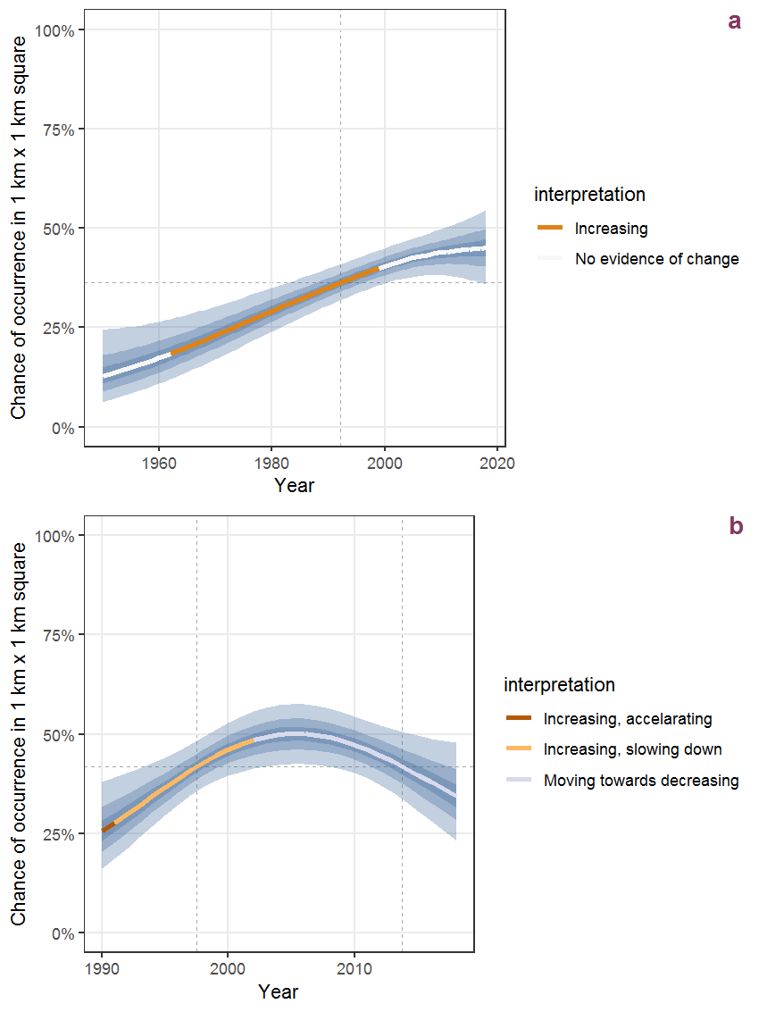
Figure F.13: Effect of year on the probability of Centaurium pulchellum (Sw.) Druce presence in 1 km x 1 km squares where the species has been observed at least once. The fitted line shows the sum of the overall mean (the intercept), a conditional effect of list-length equal to 130 and the year-smoother. The vertical dashed lines indicate the year(s) where the year-smoother is zero. The 95% confidence band is shown in grey (including the variability around the intercept and the smoother). a: 1950 - 2018, b: 1990 - 2018.
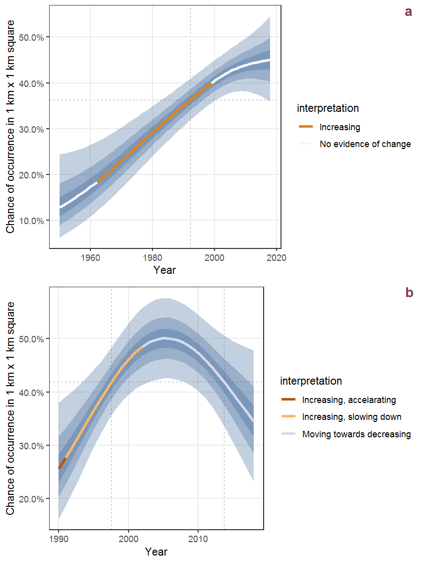
Figure F.14: The same as F.13, but the vertical axis is scaled to the range of the predicted values such that relative changes can be seen more easily. a: 1950 - 2018, b: 1990 - 2018.
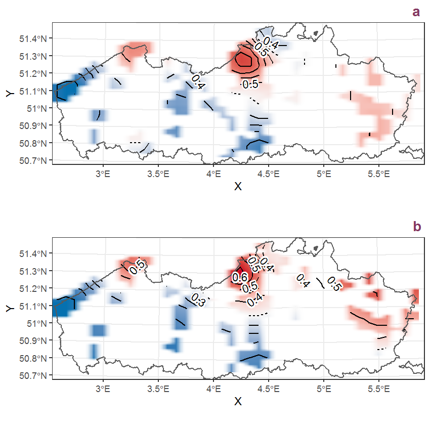
Figure F.15: Visualisation of the spatial smooth effect on the probability of Centaurium pulchellum (Sw.) Druce presence in 1 km x 1 km squares where the species has been observed at least once. The probabilities (values on the contour lines) are conditional on the final year of observation and a list-length equal to 130. The dashed contour line demarcates zones where the species is expected to be more prevalent (red shades) from zones where the species is less prevalent (blue shades). a: 1950 - 2018, b: 1990 - 2018.
F.6 Ceratocapnos claviculata (L.) Lidén
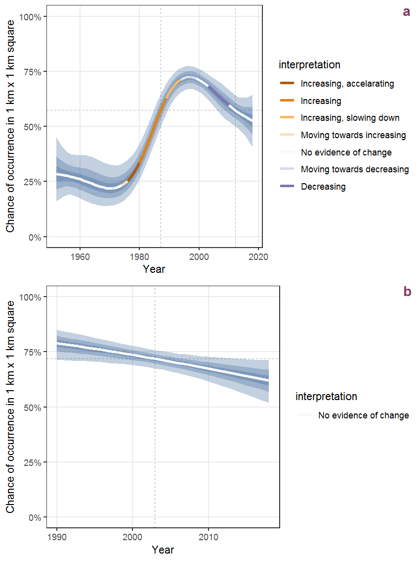
Figure F.16: Effect of year on the probability of Ceratocapnos claviculata (L.) Lidén presence in 1 km x 1 km squares where the species has been observed at least once. The fitted line shows the sum of the overall mean (the intercept), a conditional effect of list-length equal to 130 and the year-smoother. The vertical dashed lines indicate the year(s) where the year-smoother is zero. The 95% confidence band is shown in grey (including the variability around the intercept and the smoother). a: 1950 - 2018, b: 1990 - 2018.
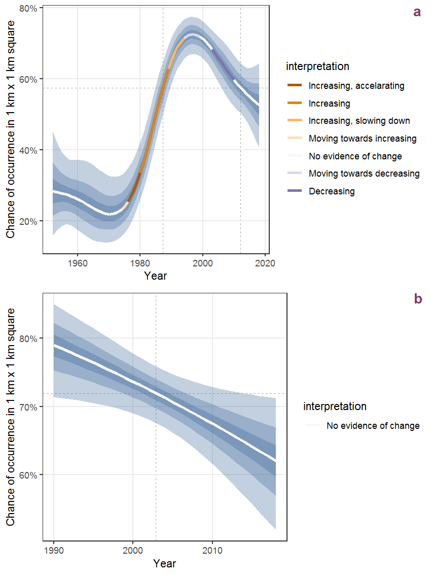
Figure F.17: The same as F.16, but the vertical axis is scaled to the range of the predicted values such that relative changes can be seen more easily. a: 1950 - 2018, b: 1990 - 2018.
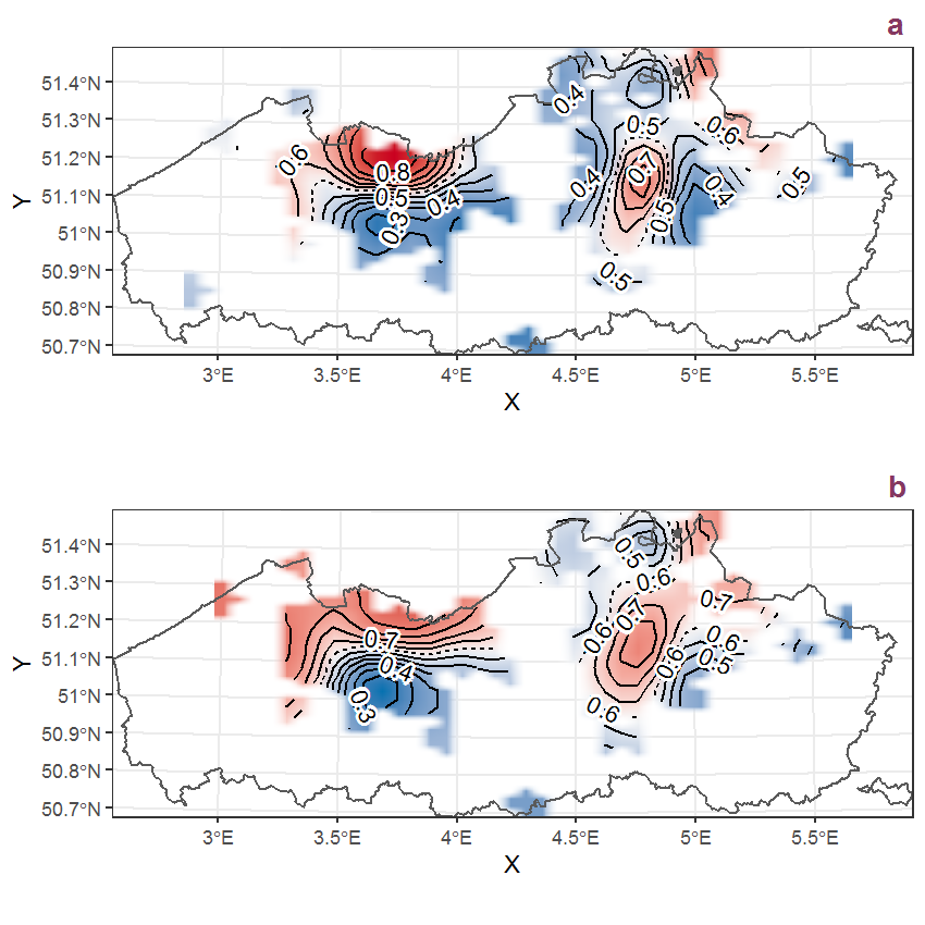
Figure F.18: Visualisation of the spatial smooth effect on the probability of Ceratocapnos claviculata (L.) Lidén presence in 1 km x 1 km squares where the species has been observed at least once. The probabilities (values on the contour lines) are conditional on the final year of observation and a list-length equal to 130. The dashed contour line demarcates zones where the species is expected to be more prevalent (red shades) from zones where the species is less prevalent (blue shades). a: 1950 - 2018, b: 1990 - 2018.
F.7 Cerastium arvense L.
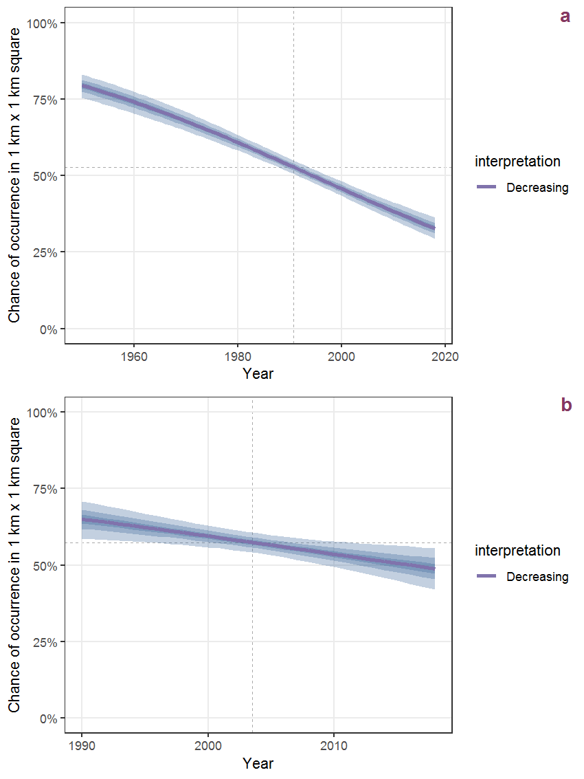
Figure F.19: Effect of year on the probability of Cerastium arvense L. presence in 1 km x 1 km squares where the species has been observed at least once. The fitted line shows the sum of the overall mean (the intercept), a conditional effect of list-length equal to 130 and the year-smoother. The vertical dashed lines indicate the year(s) where the year-smoother is zero. The 95% confidence band is shown in grey (including the variability around the intercept and the smoother). a: 1950 - 2018, b: 1990 - 2018.
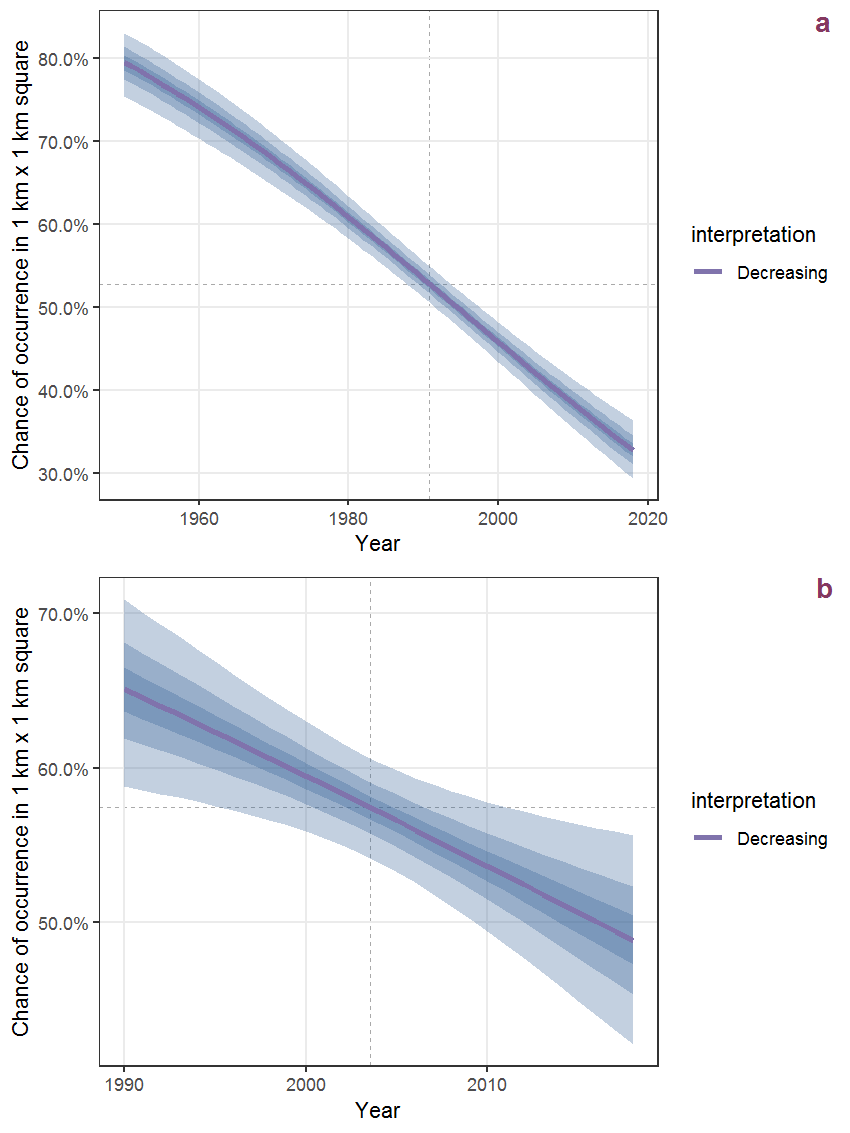
Figure F.20: The same as F.19, but the vertical axis is scaled to the range of the predicted values such that relative changes can be seen more easily. a: 1950 - 2018, b: 1990 - 2018.
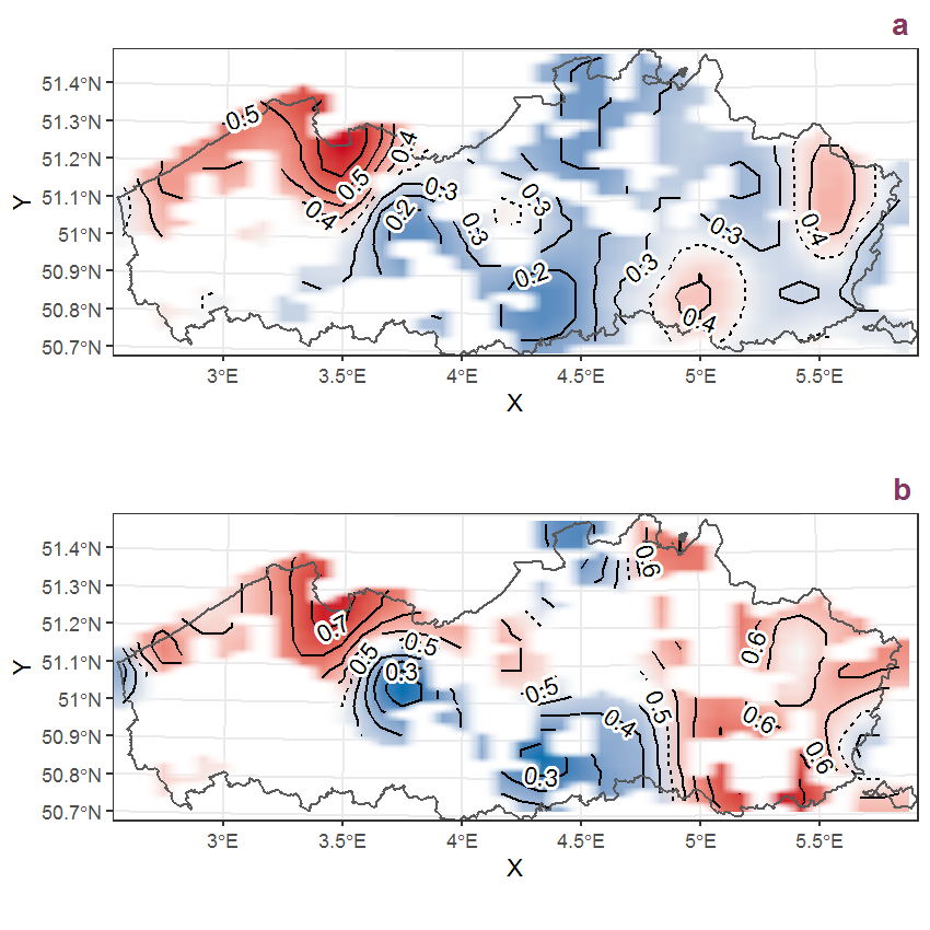
Figure F.21: Visualisation of the spatial smooth effect on the probability of Cerastium arvense L. presence in 1 km x 1 km squares where the species has been observed at least once. The probabilities (values on the contour lines) are conditional on the final year of observation and a list-length equal to 130. The dashed contour line demarcates zones where the species is expected to be more prevalent (red shades) from zones where the species is less prevalent (blue shades). a: 1950 - 2018, b: 1990 - 2018.
F.8 Cerastium fontanum Baumg.
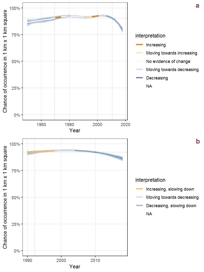
Figure F.22: Effect of year on the probability of Cerastium fontanum Baumg. presence in 1 km x 1 km squares where the species has been observed at least once. The fitted line shows the sum of the overall mean (the intercept), a conditional effect of list-length equal to 130 and the year-smoother. The vertical dashed lines indicate the year(s) where the year-smoother is zero. The 95% confidence band is shown in grey (including the variability around the intercept and the smoother). a: 1950 - 2018, b: 1990 - 2018.
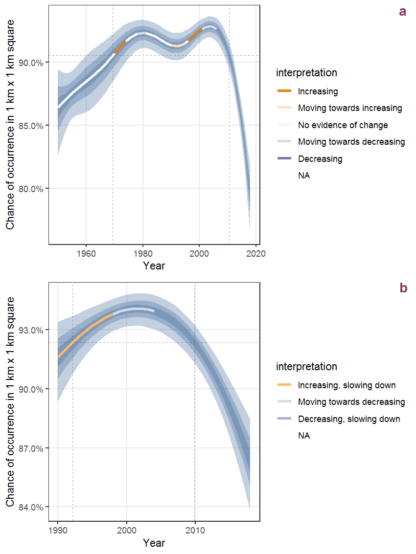
Figure F.23: The same as F.22, but the vertical axis is scaled to the range of the predicted values such that relative changes can be seen more easily. a: 1950 - 2018, b: 1990 - 2018.
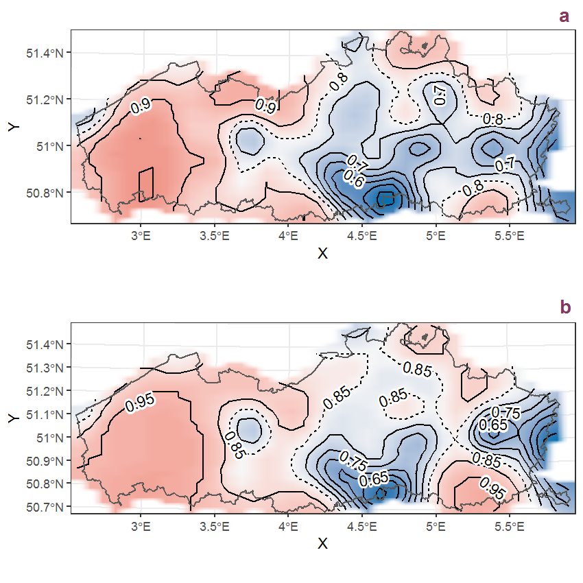
Figure F.24: Visualisation of the spatial smooth effect on the probability of Cerastium fontanum Baumg. presence in 1 km x 1 km squares where the species has been observed at least once. The probabilities (values on the contour lines) are conditional on the final year of observation and a list-length equal to 130. The dashed contour line demarcates zones where the species is expected to be more prevalent (red shades) from zones where the species is less prevalent (blue shades). a: 1950 - 2018, b: 1990 - 2018.
F.9 Cerastium glomeratum Thuill.
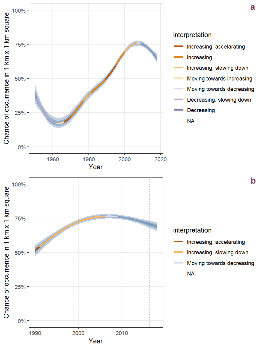
Figure F.25: Effect of year on the probability of Cerastium glomeratum Thuill. presence in 1 km x 1 km squares where the species has been observed at least once. The fitted line shows the sum of the overall mean (the intercept), a conditional effect of list-length equal to 130 and the year-smoother. The vertical dashed lines indicate the year(s) where the year-smoother is zero. The 95% confidence band is shown in grey (including the variability around the intercept and the smoother). a: 1950 - 2018, b: 1990 - 2018.
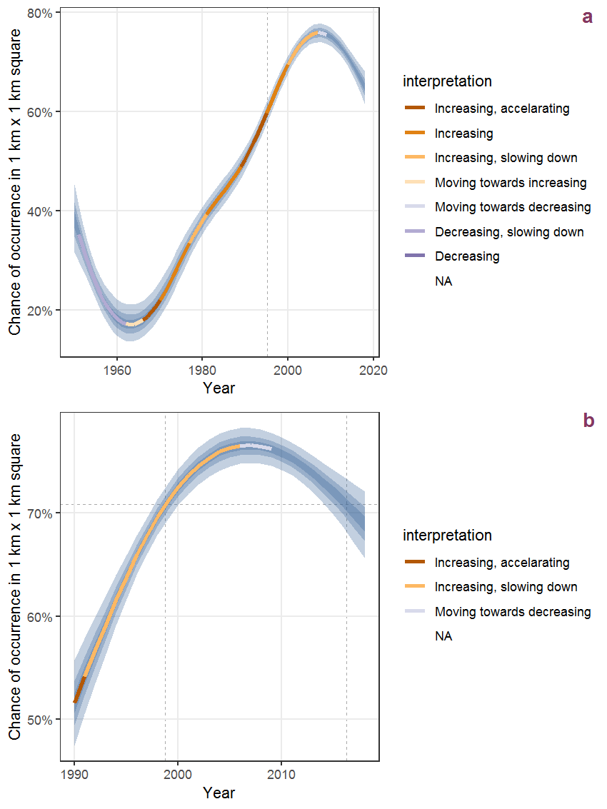
Figure F.26: The same as F.25, but the vertical axis is scaled to the range of the predicted values such that relative changes can be seen more easily. a: 1950 - 2018, b: 1990 - 2018.
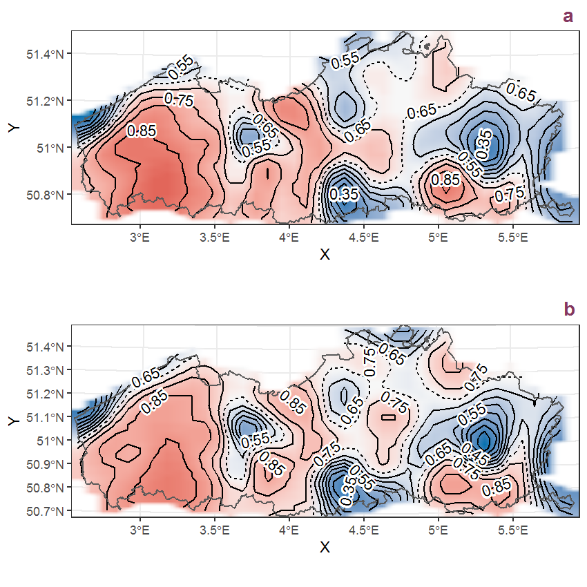
Figure F.27: Visualisation of the spatial smooth effect on the probability of Cerastium glomeratum Thuill. presence in 1 km x 1 km squares where the species has been observed at least once. The probabilities (values on the contour lines) are conditional on the final year of observation and a list-length equal to 130. The dashed contour line demarcates zones where the species is expected to be more prevalent (red shades) from zones where the species is less prevalent (blue shades). a: 1950 - 2018, b: 1990 - 2018.
F.10 Cerastium semidecandrum L.
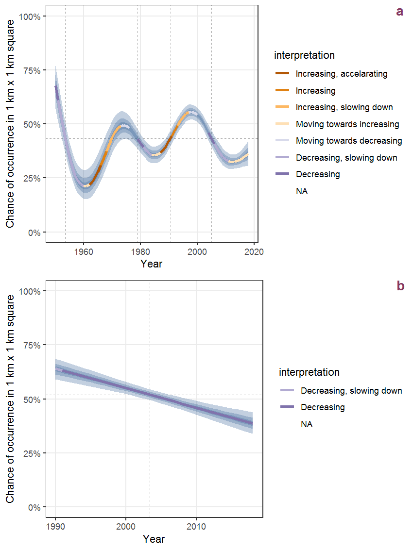
Figure F.28: Effect of year on the probability of Cerastium semidecandrum L. presence in 1 km x 1 km squares where the species has been observed at least once. The fitted line shows the sum of the overall mean (the intercept), a conditional effect of list-length equal to 130 and the year-smoother. The vertical dashed lines indicate the year(s) where the year-smoother is zero. The 95% confidence band is shown in grey (including the variability around the intercept and the smoother). a: 1950 - 2018, b: 1990 - 2018.
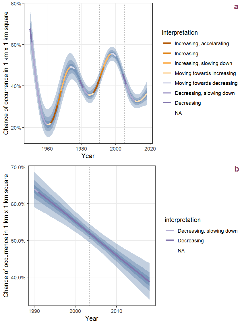
Figure F.29: The same as F.28, but the vertical axis is scaled to the range of the predicted values such that relative changes can be seen more easily. a: 1950 - 2018, b: 1990 - 2018.
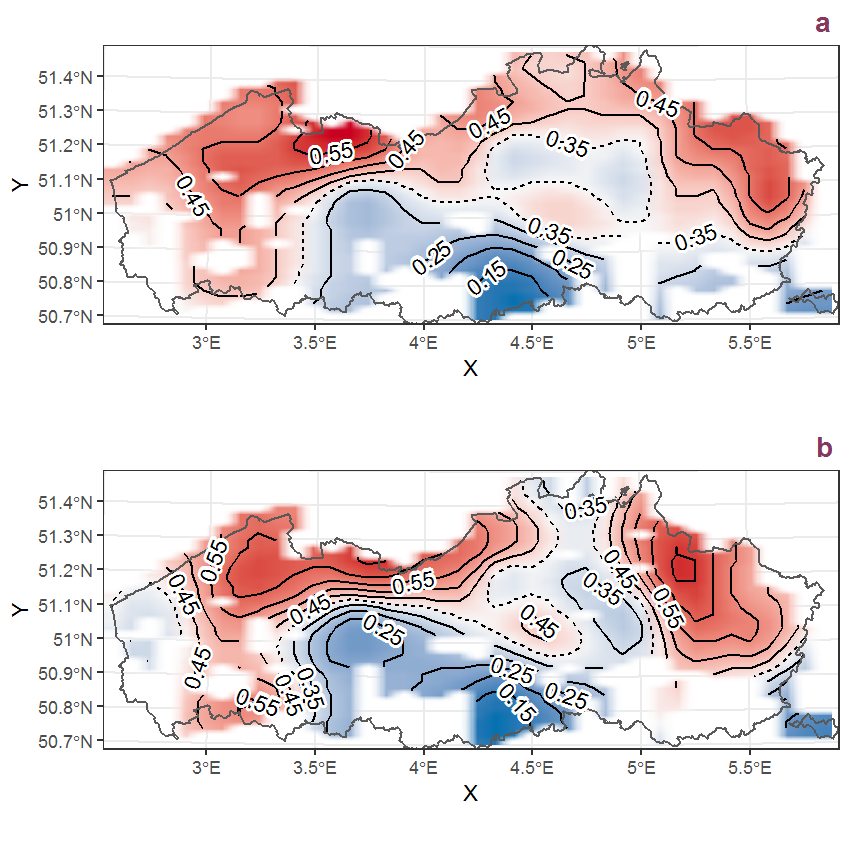
Figure F.30: Visualisation of the spatial smooth effect on the probability of Cerastium semidecandrum L. presence in 1 km x 1 km squares where the species has been observed at least once. The probabilities (values on the contour lines) are conditional on the final year of observation and a list-length equal to 130. The dashed contour line demarcates zones where the species is expected to be more prevalent (red shades) from zones where the species is less prevalent (blue shades). a: 1950 - 2018, b: 1990 - 2018.
F.11 Cerastium tomentosum L.
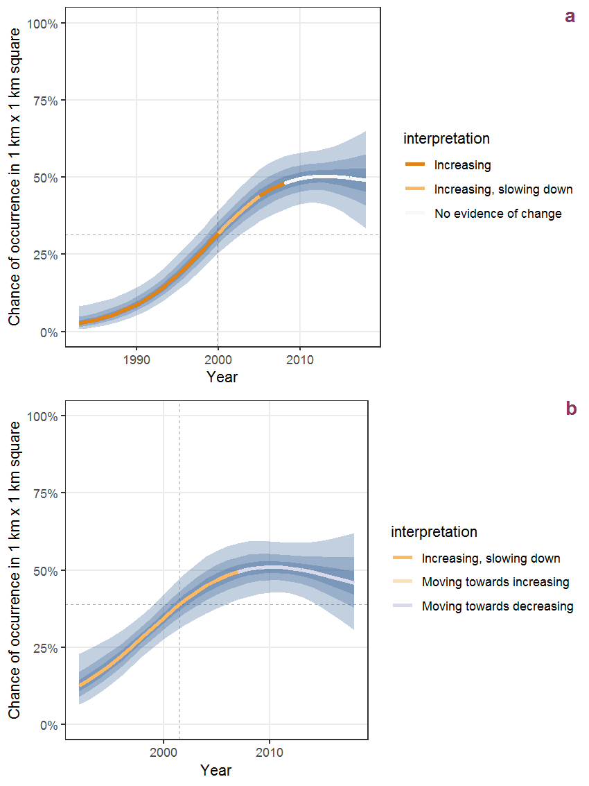
Figure F.31: Effect of year on the probability of Cerastium tomentosum L. presence in 1 km x 1 km squares where the species has been observed at least once. The fitted line shows the sum of the overall mean (the intercept), a conditional effect of list-length equal to 130 and the year-smoother. The vertical dashed lines indicate the year(s) where the year-smoother is zero. The 95% confidence band is shown in grey (including the variability around the intercept and the smoother). a: 1950 - 2018, b: 1990 - 2018.
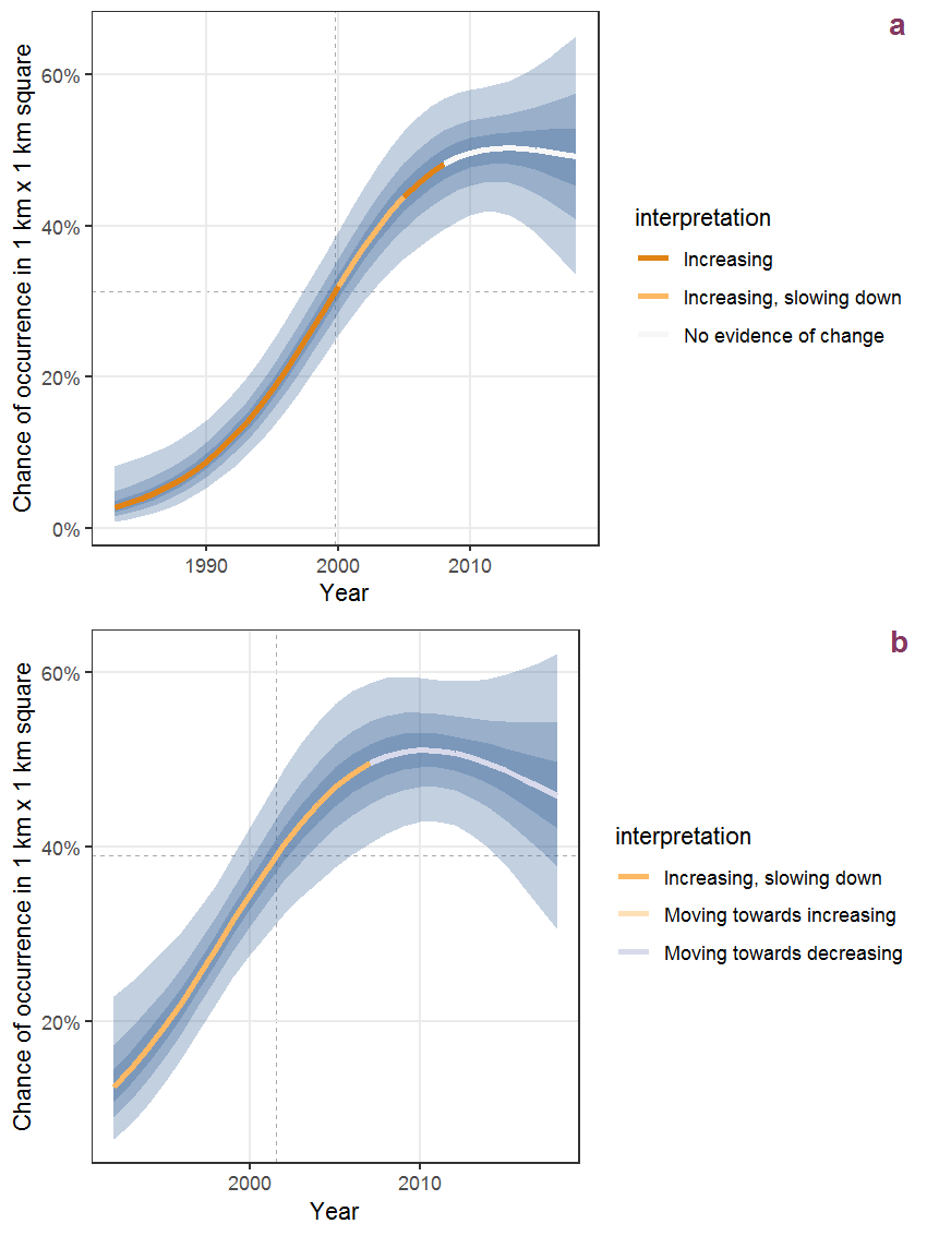
Figure F.32: The same as F.31, but the vertical axis is scaled to the range of the predicted values such that relative changes can be seen more easily. a: 1950 - 2018, b: 1990 - 2018.
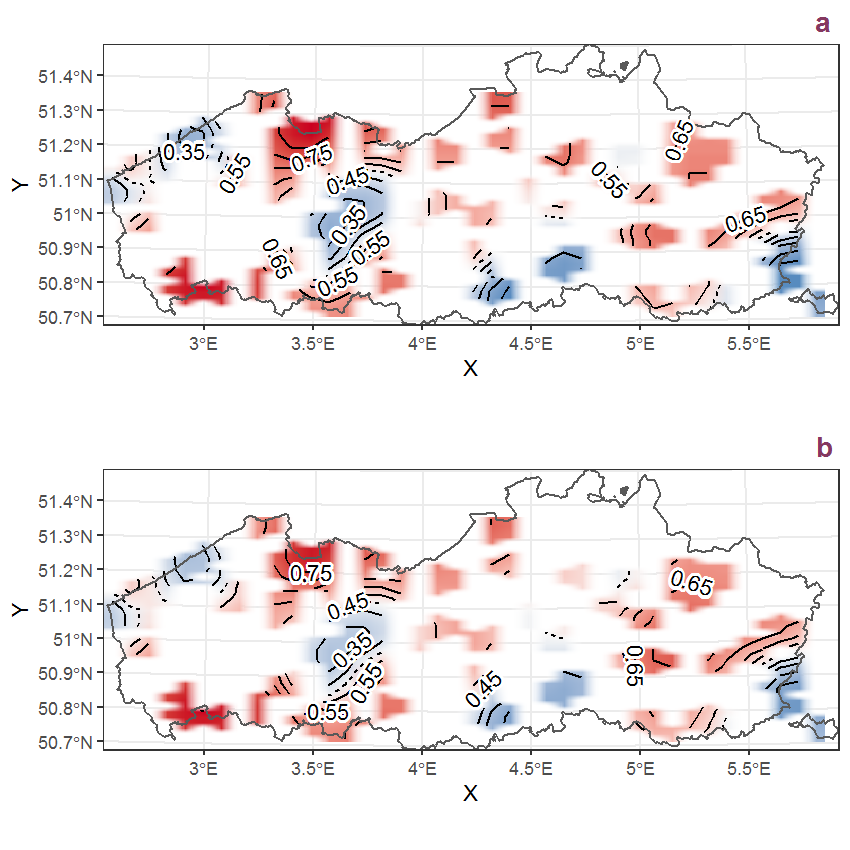
Figure F.33: Visualisation of the spatial smooth effect on the probability of Cerastium tomentosum L. presence in 1 km x 1 km squares where the species has been observed at least once. The probabilities (values on the contour lines) are conditional on the final year of observation and a list-length equal to 130. The dashed contour line demarcates zones where the species is expected to be more prevalent (red shades) from zones where the species is less prevalent (blue shades). a: 1950 - 2018, b: 1990 - 2018.
F.12 Ceratophyllum demersum L.
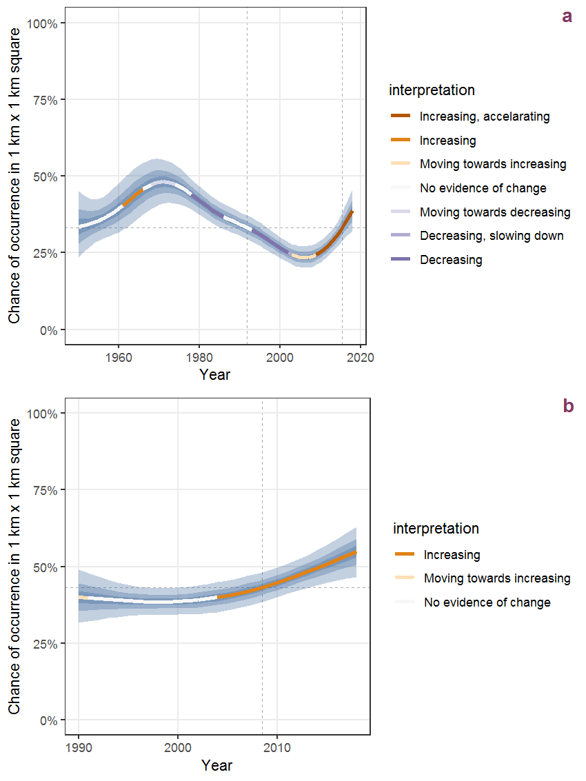
Figure F.34: Effect of year on the probability of Ceratophyllum demersum L. presence in 1 km x 1 km squares where the species has been observed at least once. The fitted line shows the sum of the overall mean (the intercept), a conditional effect of list-length equal to 130 and the year-smoother. The vertical dashed lines indicate the year(s) where the year-smoother is zero. The 95% confidence band is shown in grey (including the variability around the intercept and the smoother). a: 1950 - 2018, b: 1990 - 2018.
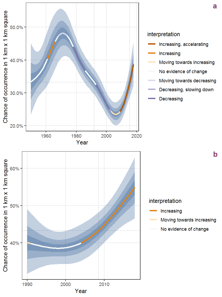
Figure F.35: The same as F.34, but the vertical axis is scaled to the range of the predicted values such that relative changes can be seen more easily. a: 1950 - 2018, b: 1990 - 2018.
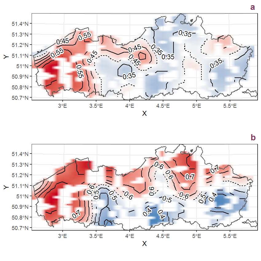
Figure F.36: Visualisation of the spatial smooth effect on the probability of Ceratophyllum demersum L. presence in 1 km x 1 km squares where the species has been observed at least once. The probabilities (values on the contour lines) are conditional on the final year of observation and a list-length equal to 130. The dashed contour line demarcates zones where the species is expected to be more prevalent (red shades) from zones where the species is less prevalent (blue shades). a: 1950 - 2018, b: 1990 - 2018.
F.13 Chaenorrhinum minus (L.) Lange
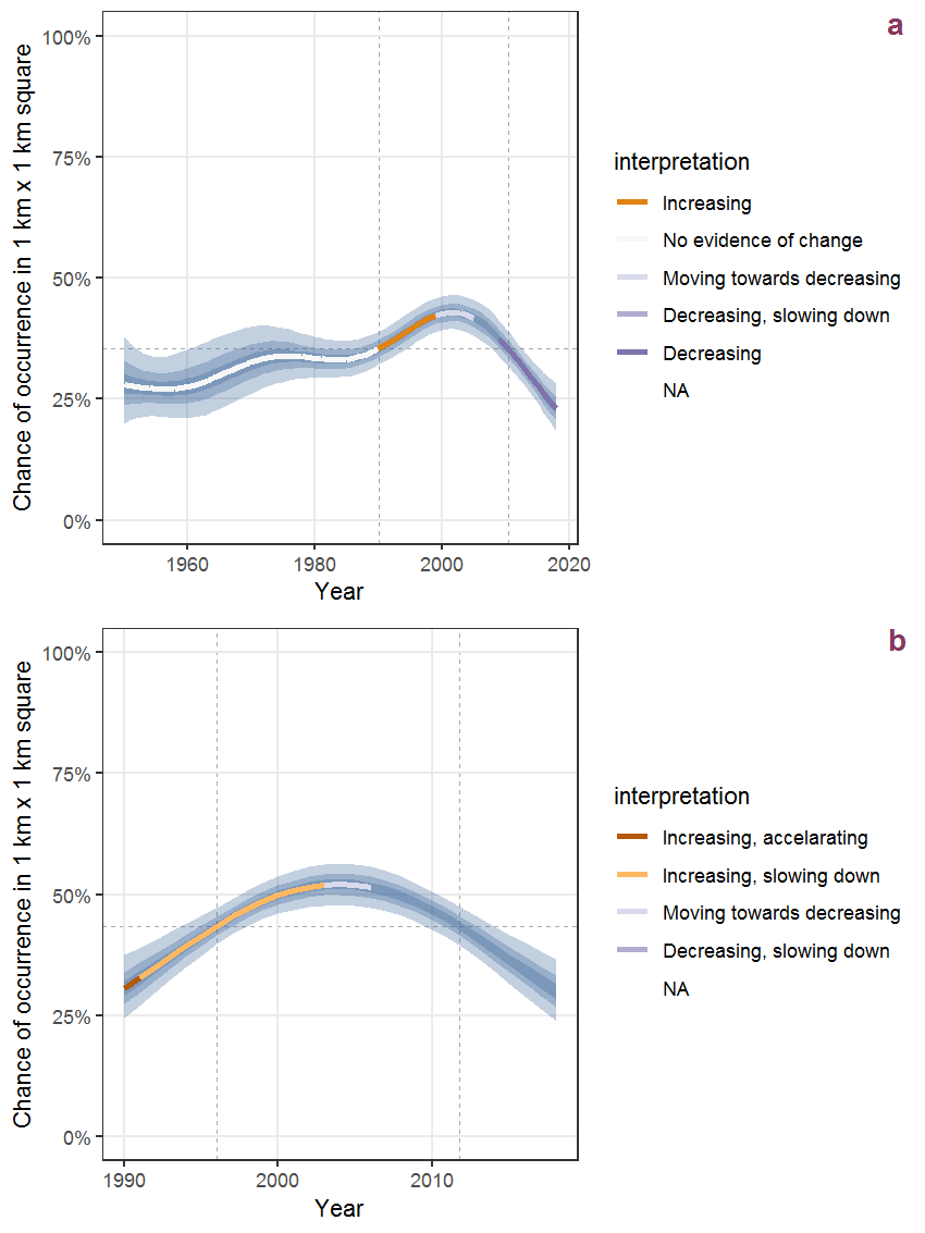
Figure F.37: Effect of year on the probability of Chaenorrhinum minus (L.) Lange presence in 1 km x 1 km squares where the species has been observed at least once. The fitted line shows the sum of the overall mean (the intercept), a conditional effect of list-length equal to 130 and the year-smoother. The vertical dashed lines indicate the year(s) where the year-smoother is zero. The 95% confidence band is shown in grey (including the variability around the intercept and the smoother). a: 1950 - 2018, b: 1990 - 2018.
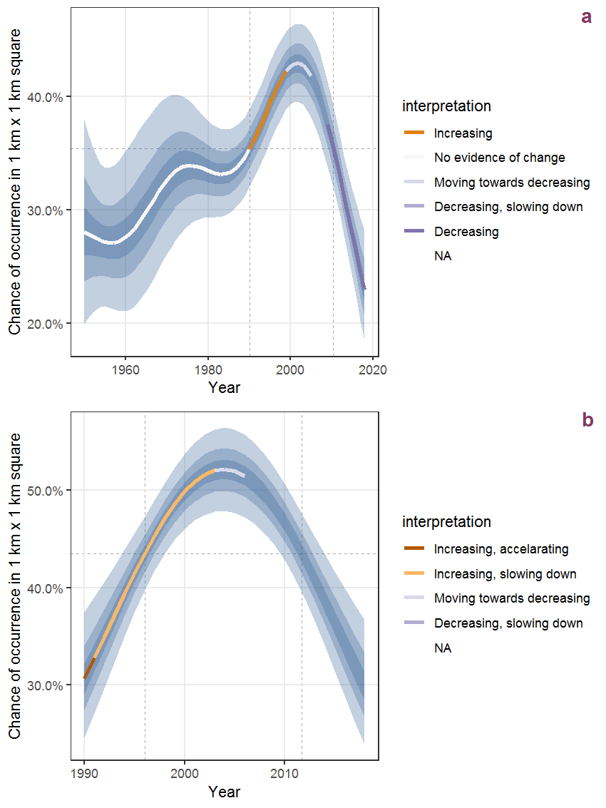
Figure F.38: The same as F.37, but the vertical axis is scaled to the range of the predicted values such that relative changes can be seen more easily. a: 1950 - 2018, b: 1990 - 2018.
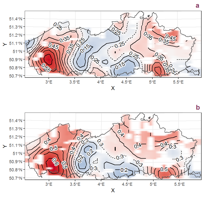
Figure F.39: Visualisation of the spatial smooth effect on the probability of Chaenorrhinum minus (L.) Lange presence in 1 km x 1 km squares where the species has been observed at least once. The probabilities (values on the contour lines) are conditional on the final year of observation and a list-length equal to 130. The dashed contour line demarcates zones where the species is expected to be more prevalent (red shades) from zones where the species is less prevalent (blue shades). a: 1950 - 2018, b: 1990 - 2018.
F.14 Chaerophyllum temulum L.
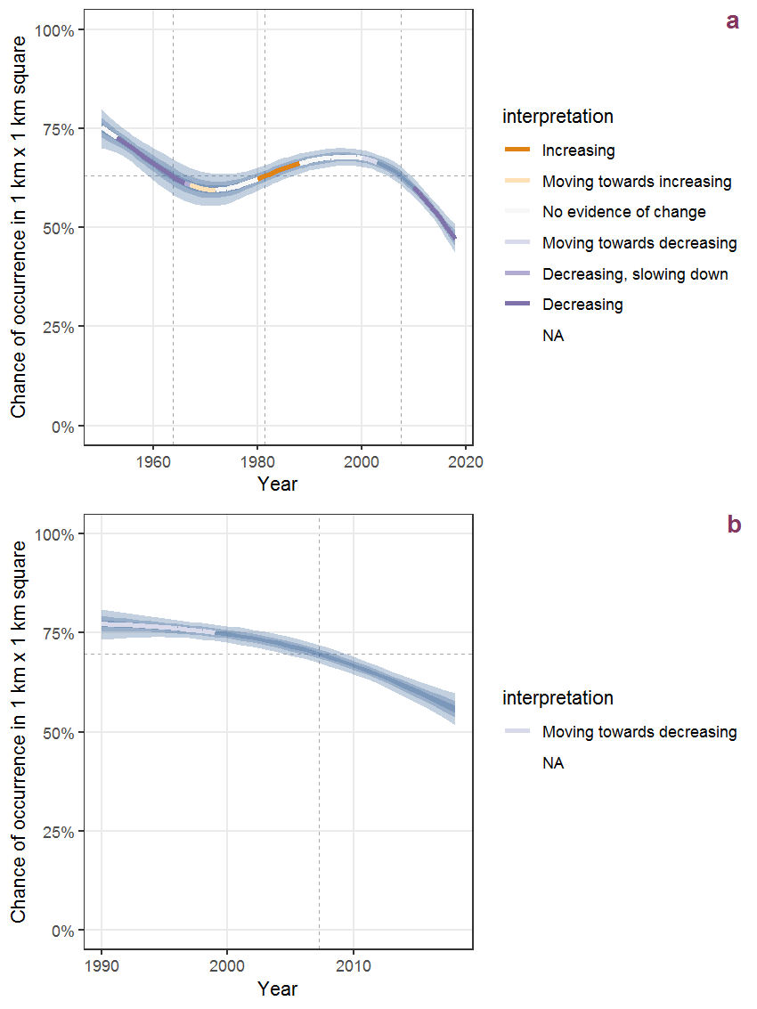
Figure F.40: Effect of year on the probability of Chaerophyllum temulum L. presence in 1 km x 1 km squares where the species has been observed at least once. The fitted line shows the sum of the overall mean (the intercept), a conditional effect of list-length equal to 130 and the year-smoother. The vertical dashed lines indicate the year(s) where the year-smoother is zero. The 95% confidence band is shown in grey (including the variability around the intercept and the smoother). a: 1950 - 2018, b: 1990 - 2018.
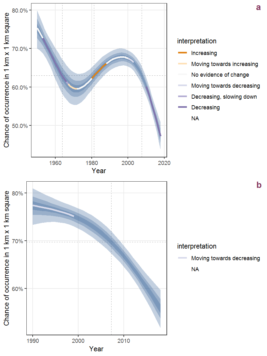
Figure F.41: The same as F.40, but the vertical axis is scaled to the range of the predicted values such that relative changes can be seen more easily. a: 1950 - 2018, b: 1990 - 2018.
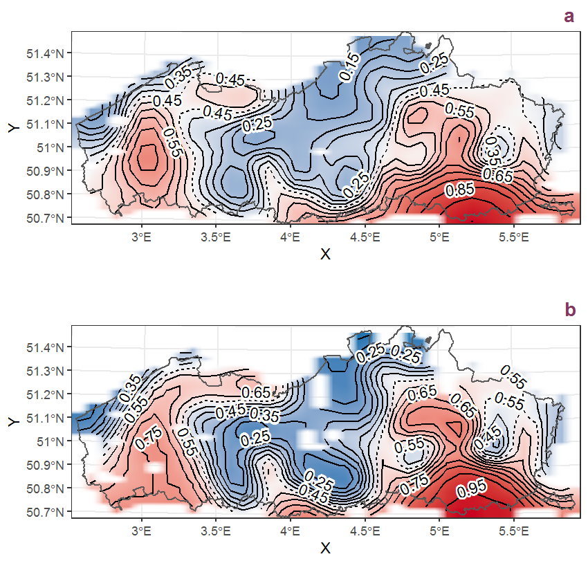
Figure F.42: Visualisation of the spatial smooth effect on the probability of Chaerophyllum temulum L. presence in 1 km x 1 km squares where the species has been observed at least once. The probabilities (values on the contour lines) are conditional on the final year of observation and a list-length equal to 130. The dashed contour line demarcates zones where the species is expected to be more prevalent (red shades) from zones where the species is less prevalent (blue shades). a: 1950 - 2018, b: 1990 - 2018.
F.15 Epilobium angustifolium L.
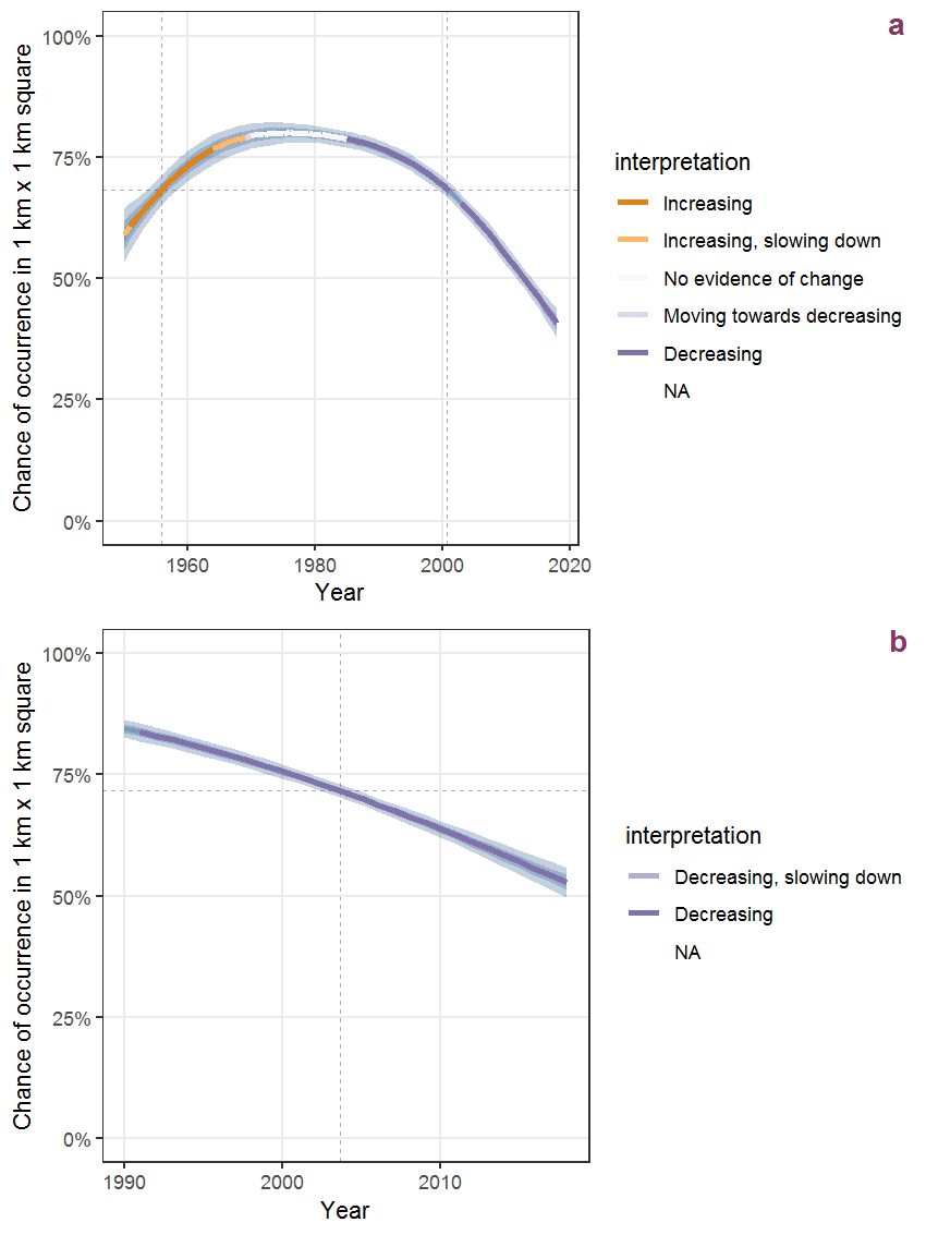
Figure F.43: Effect of year on the probability of Epilobium angustifolium L. presence in 1 km x 1 km squares where the species has been observed at least once. The fitted line shows the sum of the overall mean (the intercept), a conditional effect of list-length equal to 130 and the year-smoother. The vertical dashed lines indicate the year(s) where the year-smoother is zero. The 95% confidence band is shown in grey (including the variability around the intercept and the smoother). a: 1950 - 2018, b: 1990 - 2018.
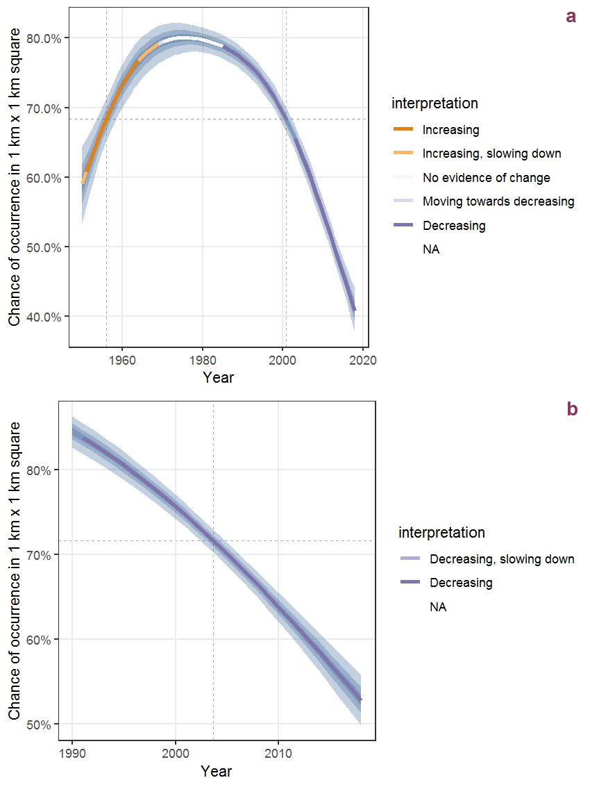
Figure F.44: The same as F.43, but the vertical axis is scaled to the range of the predicted values such that relative changes can be seen more easily. a: 1950 - 2018, b: 1990 - 2018.
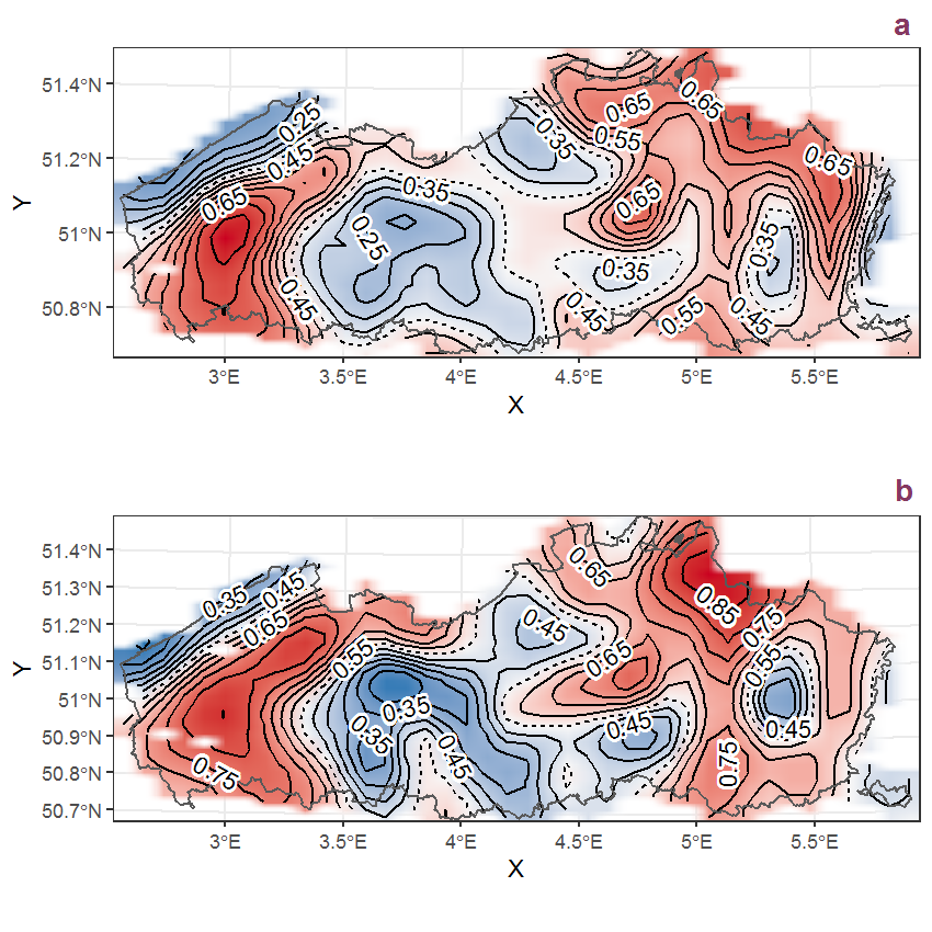
Figure F.45: Visualisation of the spatial smooth effect on the probability of Epilobium angustifolium L. presence in 1 km x 1 km squares where the species has been observed at least once. The probabilities (values on the contour lines) are conditional on the final year of observation and a list-length equal to 130. The dashed contour line demarcates zones where the species is expected to be more prevalent (red shades) from zones where the species is less prevalent (blue shades). a: 1950 - 2018, b: 1990 - 2018.
F.16 Chelidonium majus L.
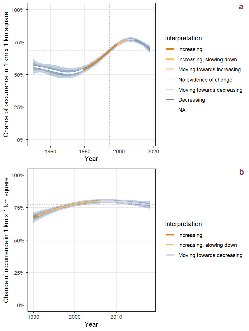
Figure F.46: Effect of year on the probability of Chelidonium majus L. presence in 1 km x 1 km squares where the species has been observed at least once. The fitted line shows the sum of the overall mean (the intercept), a conditional effect of list-length equal to 130 and the year-smoother. The vertical dashed lines indicate the year(s) where the year-smoother is zero. The 95% confidence band is shown in grey (including the variability around the intercept and the smoother). a: 1950 - 2018, b: 1990 - 2018.
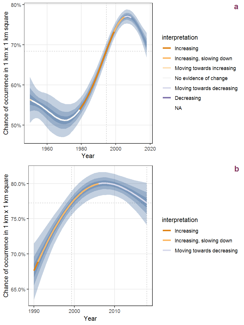
Figure F.47: The same as F.46, but the vertical axis is scaled to the range of the predicted values such that relative changes can be seen more easily. a: 1950 - 2018, b: 1990 - 2018.
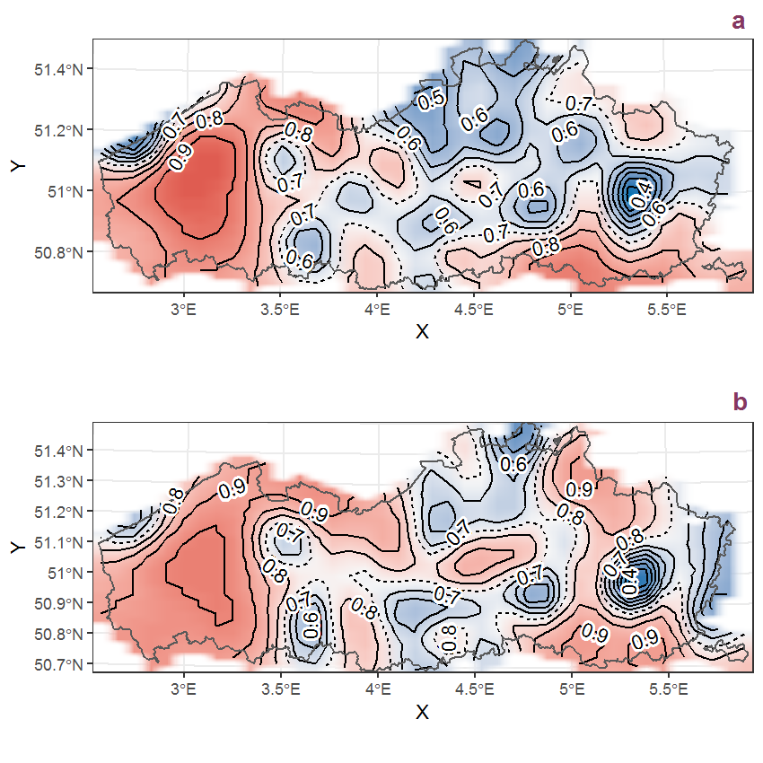
Figure F.48: Visualisation of the spatial smooth effect on the probability of Chelidonium majus L. presence in 1 km x 1 km squares where the species has been observed at least once. The probabilities (values on the contour lines) are conditional on the final year of observation and a list-length equal to 130. The dashed contour line demarcates zones where the species is expected to be more prevalent (red shades) from zones where the species is less prevalent (blue shades). a: 1950 - 2018, b: 1990 - 2018.
F.17 Chenopodium album L.
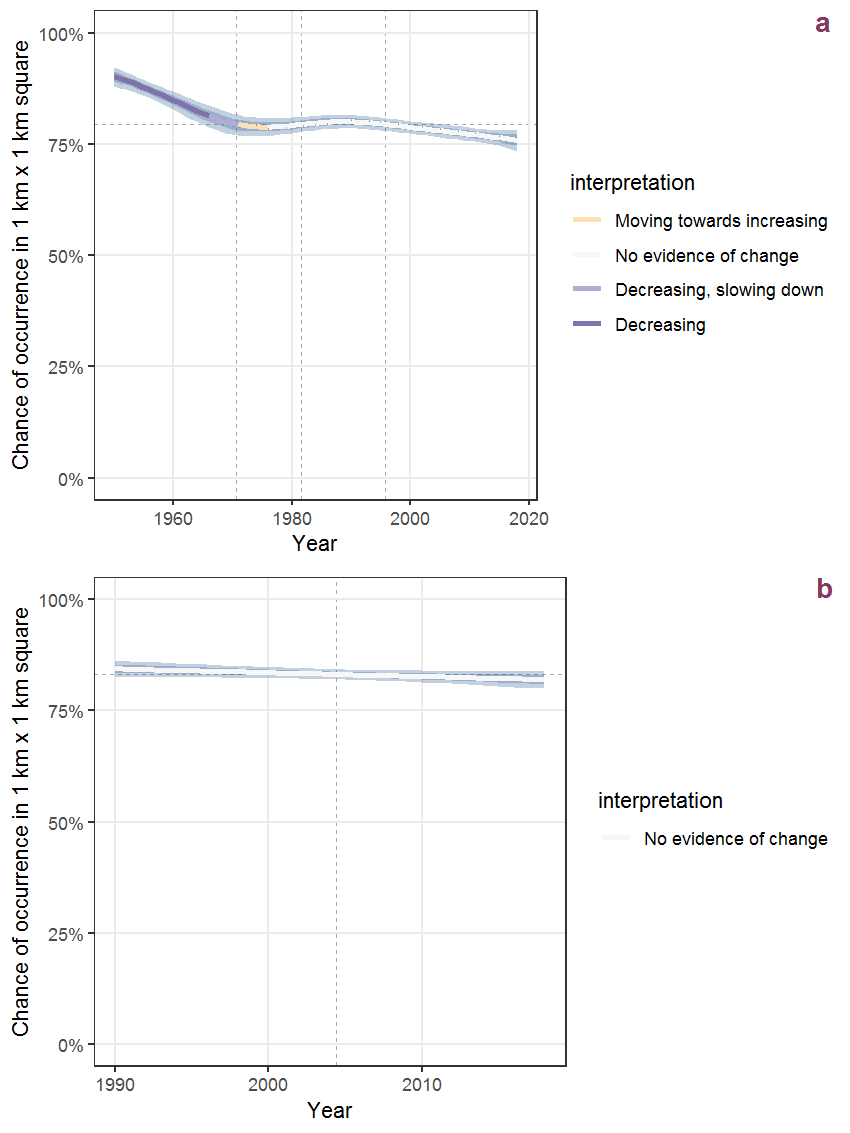
Figure F.49: Effect of year on the probability of Chenopodium album L. presence in 1 km x 1 km squares where the species has been observed at least once. The fitted line shows the sum of the overall mean (the intercept), a conditional effect of list-length equal to 130 and the year-smoother. The vertical dashed lines indicate the year(s) where the year-smoother is zero. The 95% confidence band is shown in grey (including the variability around the intercept and the smoother). a: 1950 - 2018, b: 1990 - 2018.
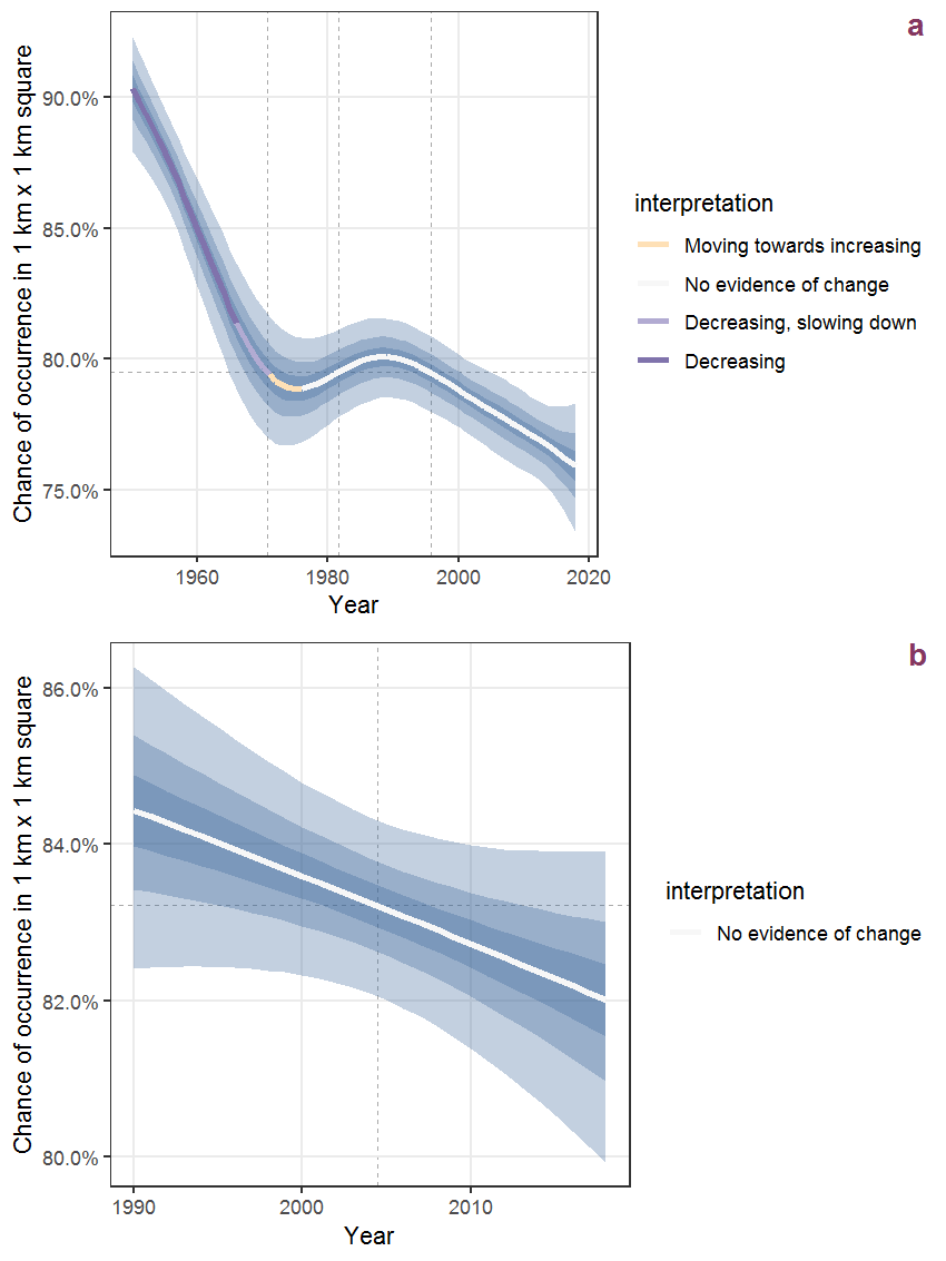
Figure F.50: The same as F.49, but the vertical axis is scaled to the range of the predicted values such that relative changes can be seen more easily. a: 1950 - 2018, b: 1990 - 2018.
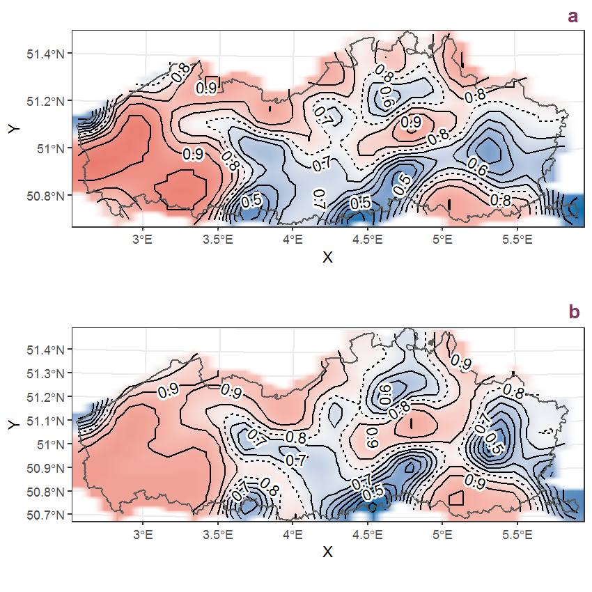
Figure F.51: Visualisation of the spatial smooth effect on the probability of Chenopodium album L. presence in 1 km x 1 km squares where the species has been observed at least once. The probabilities (values on the contour lines) are conditional on the final year of observation and a list-length equal to 130. The dashed contour line demarcates zones where the species is expected to be more prevalent (red shades) from zones where the species is less prevalent (blue shades). a: 1950 - 2018, b: 1990 - 2018.
F.18 Chenopodium ficifolium Smith
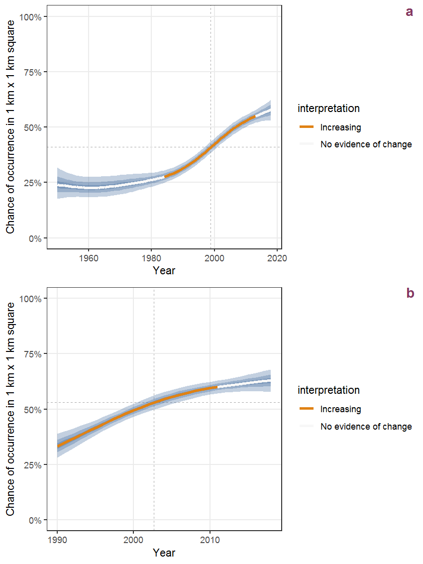
Figure F.52: Effect of year on the probability of Chenopodium ficifolium Smith presence in 1 km x 1 km squares where the species has been observed at least once. The fitted line shows the sum of the overall mean (the intercept), a conditional effect of list-length equal to 130 and the year-smoother. The vertical dashed lines indicate the year(s) where the year-smoother is zero. The 95% confidence band is shown in grey (including the variability around the intercept and the smoother). a: 1950 - 2018, b: 1990 - 2018.
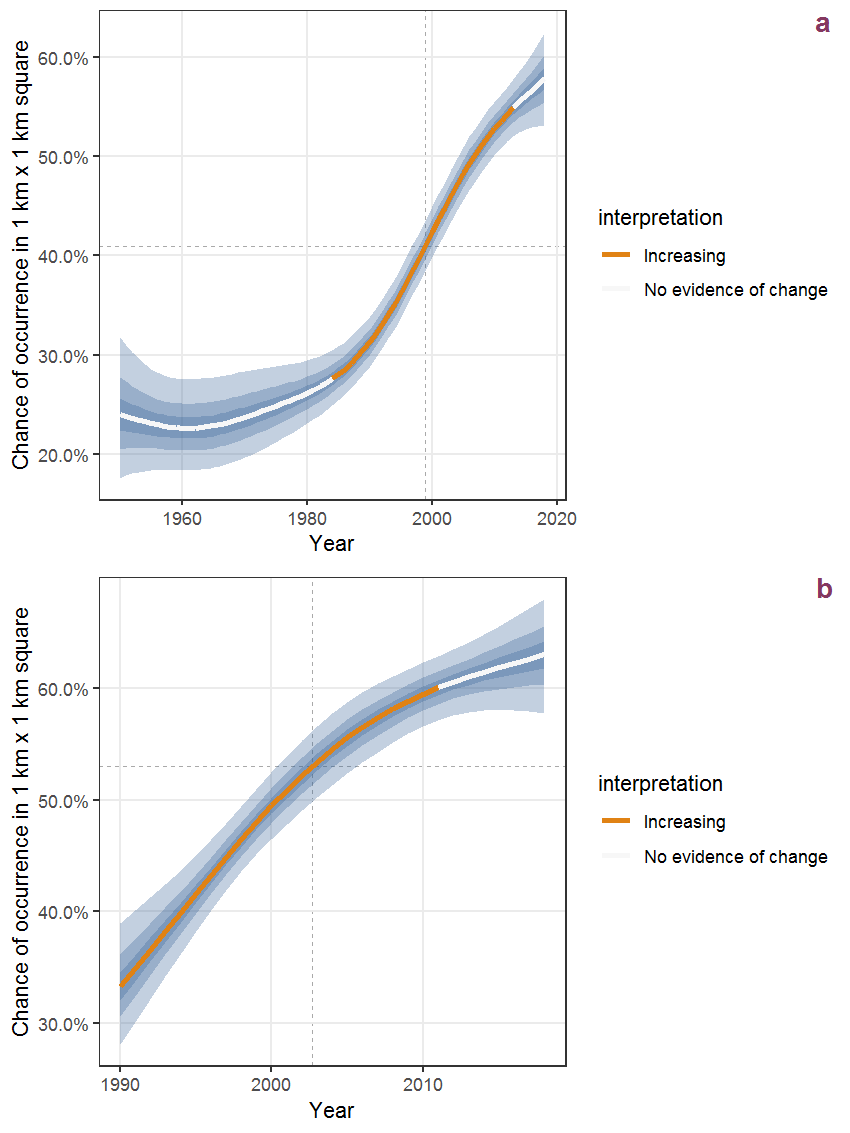
Figure F.53: The same as F.52, but the vertical axis is scaled to the range of the predicted values such that relative changes can be seen more easily. a: 1950 - 2018, b: 1990 - 2018.
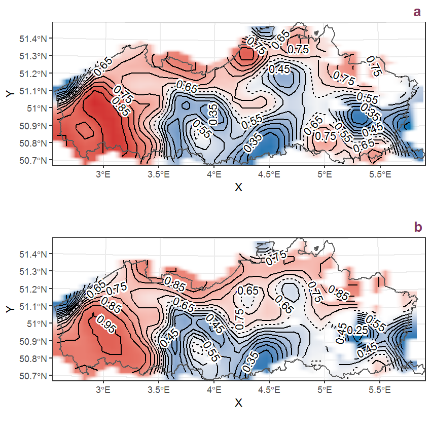
Figure F.54: Visualisation of the spatial smooth effect on the probability of Chenopodium ficifolium Smith presence in 1 km x 1 km squares where the species has been observed at least once. The probabilities (values on the contour lines) are conditional on the final year of observation and a list-length equal to 130. The dashed contour line demarcates zones where the species is expected to be more prevalent (red shades) from zones where the species is less prevalent (blue shades). a: 1950 - 2018, b: 1990 - 2018.
F.19 Chenopodium glaucum L.
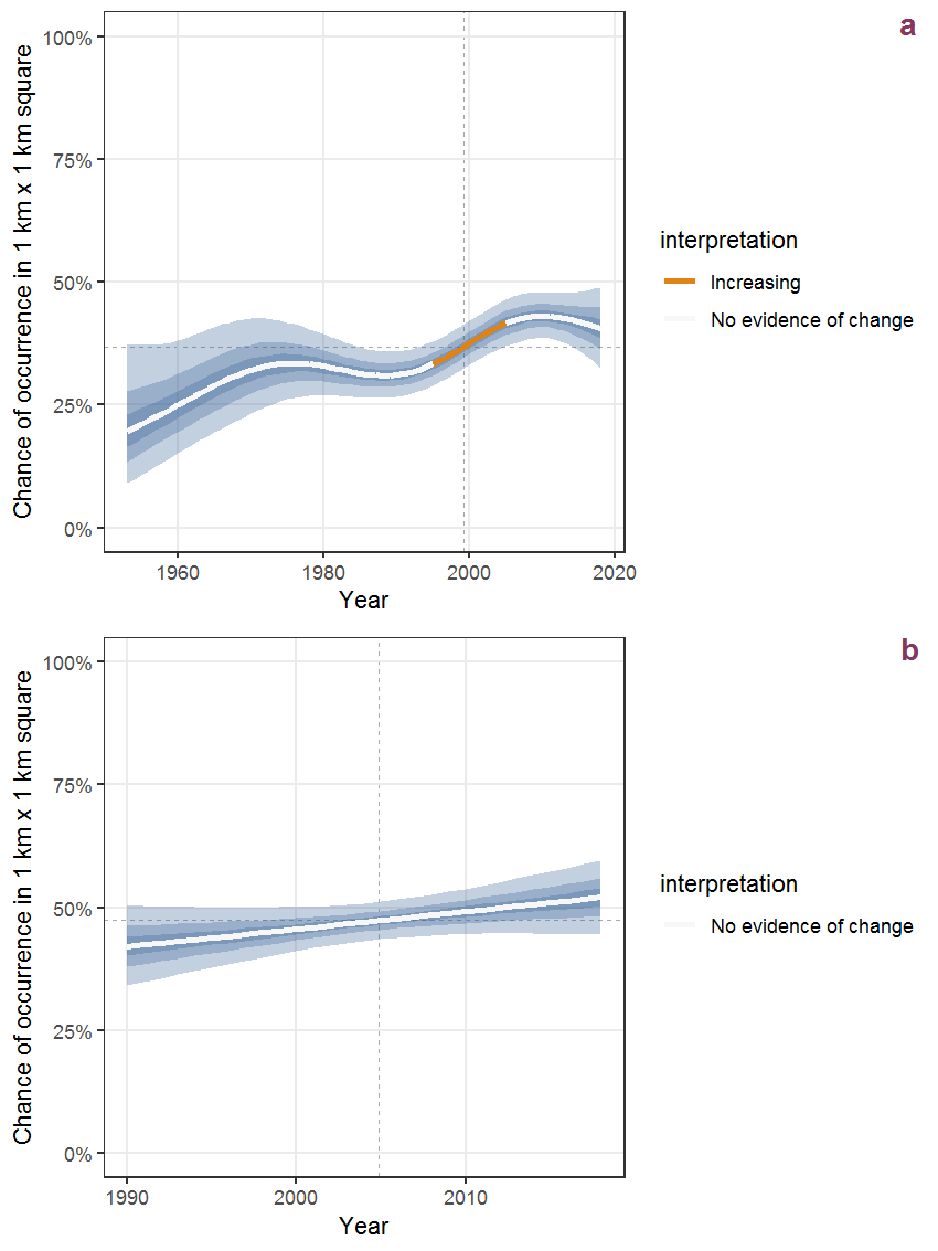
Figure F.55: Effect of year on the probability of Chenopodium glaucum L. presence in 1 km x 1 km squares where the species has been observed at least once. The fitted line shows the sum of the overall mean (the intercept), a conditional effect of list-length equal to 130 and the year-smoother. The vertical dashed lines indicate the year(s) where the year-smoother is zero. The 95% confidence band is shown in grey (including the variability around the intercept and the smoother). a: 1950 - 2018, b: 1990 - 2018.
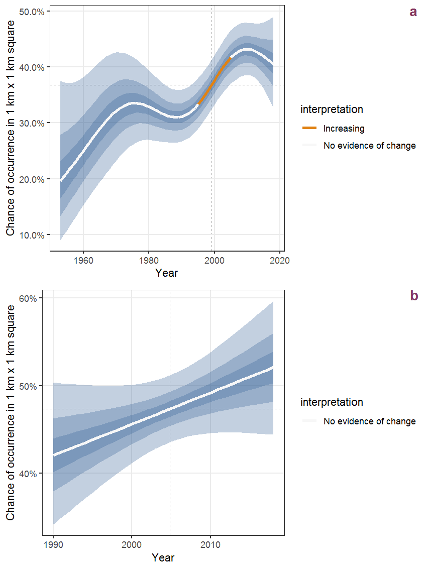
Figure F.56: The same as F.55, but the vertical axis is scaled to the range of the predicted values such that relative changes can be seen more easily. a: 1950 - 2018, b: 1990 - 2018.
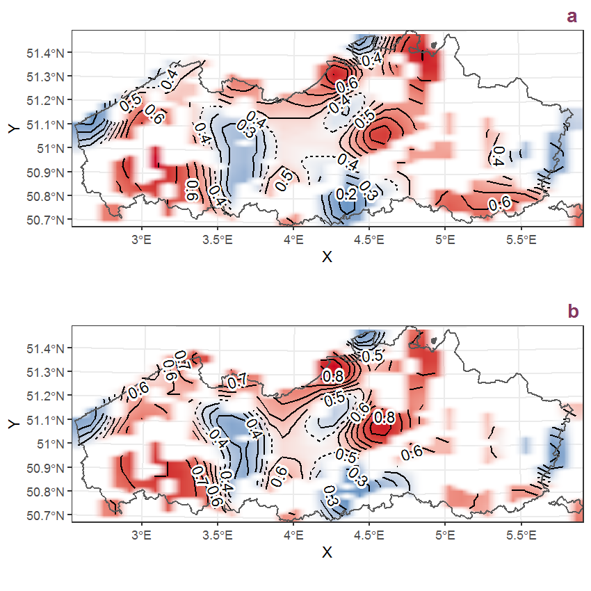
Figure F.57: Visualisation of the spatial smooth effect on the probability of Chenopodium glaucum L. presence in 1 km x 1 km squares where the species has been observed at least once. The probabilities (values on the contour lines) are conditional on the final year of observation and a list-length equal to 130. The dashed contour line demarcates zones where the species is expected to be more prevalent (red shades) from zones where the species is less prevalent (blue shades). a: 1950 - 2018, b: 1990 - 2018.
F.20 Chenopodium polyspermum L.
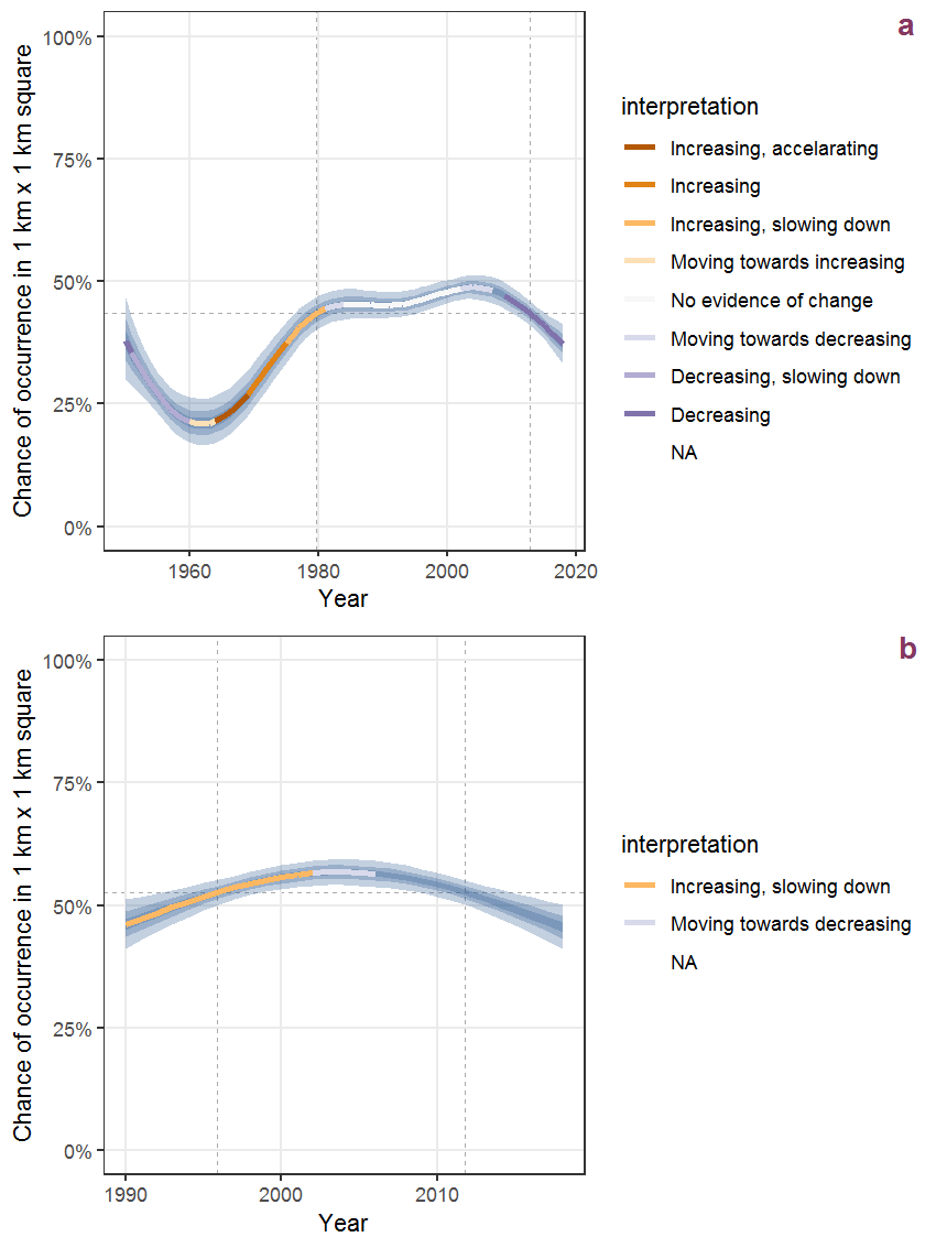
Figure F.58: Effect of year on the probability of Chenopodium polyspermum L. presence in 1 km x 1 km squares where the species has been observed at least once. The fitted line shows the sum of the overall mean (the intercept), a conditional effect of list-length equal to 130 and the year-smoother. The vertical dashed lines indicate the year(s) where the year-smoother is zero. The 95% confidence band is shown in grey (including the variability around the intercept and the smoother). a: 1950 - 2018, b: 1990 - 2018.
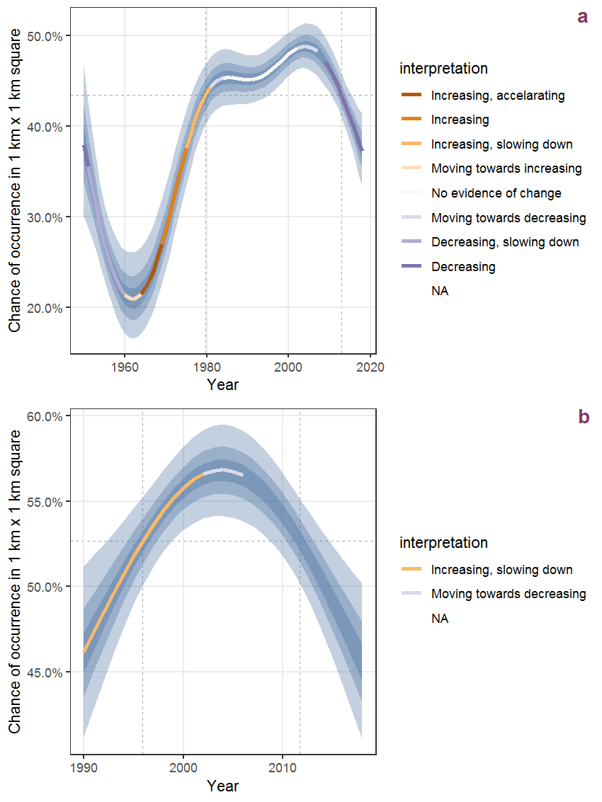
Figure F.59: The same as F.58, but the vertical axis is scaled to the range of the predicted values such that relative changes can be seen more easily. a: 1950 - 2018, b: 1990 - 2018.
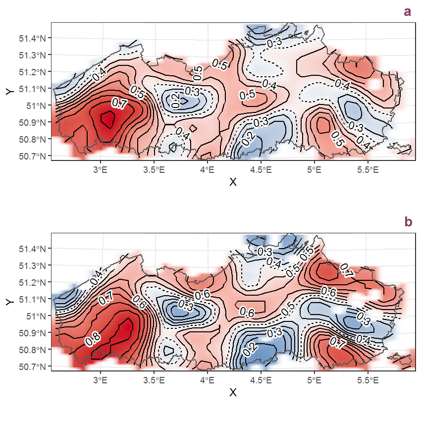
Figure F.60: Visualisation of the spatial smooth effect on the probability of Chenopodium polyspermum L. presence in 1 km x 1 km squares where the species has been observed at least once. The probabilities (values on the contour lines) are conditional on the final year of observation and a list-length equal to 130. The dashed contour line demarcates zones where the species is expected to be more prevalent (red shades) from zones where the species is less prevalent (blue shades). a: 1950 - 2018, b: 1990 - 2018.
F.21 Chenopodium rubrum L.
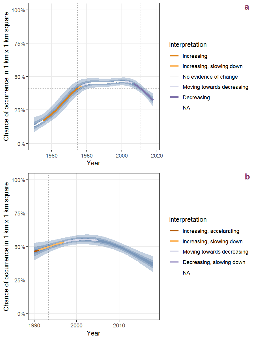
Figure F.61: Effect of year on the probability of Chenopodium rubrum L. presence in 1 km x 1 km squares where the species has been observed at least once. The fitted line shows the sum of the overall mean (the intercept), a conditional effect of list-length equal to 130 and the year-smoother. The vertical dashed lines indicate the year(s) where the year-smoother is zero. The 95% confidence band is shown in grey (including the variability around the intercept and the smoother). a: 1950 - 2018, b: 1990 - 2018.
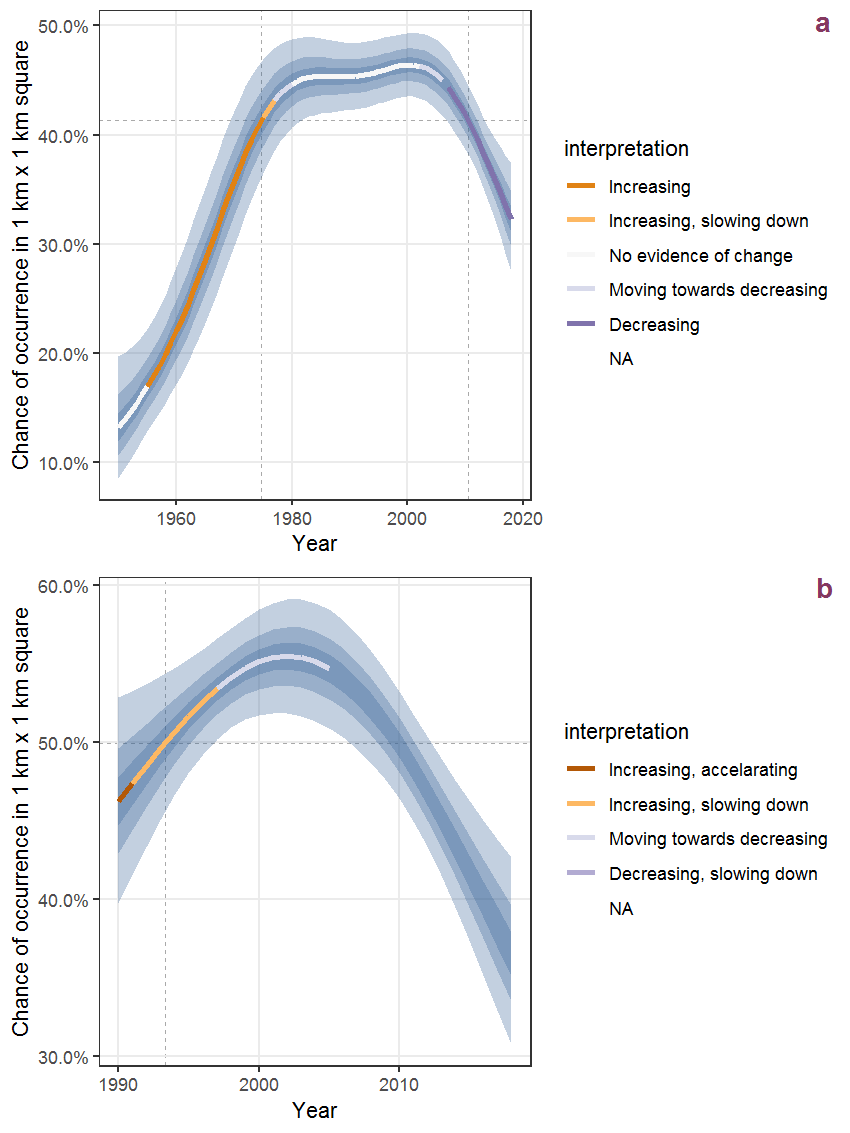
Figure F.62: The same as F.61, but the vertical axis is scaled to the range of the predicted values such that relative changes can be seen more easily. a: 1950 - 2018, b: 1990 - 2018.
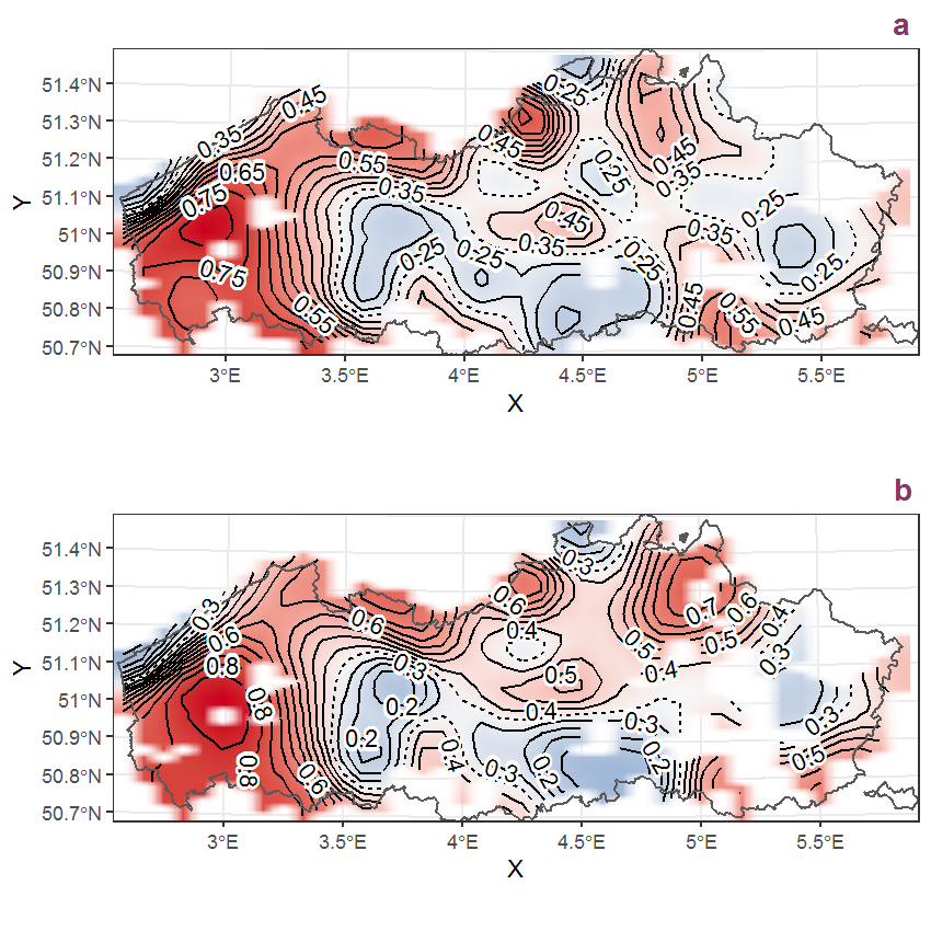
Figure F.63: Visualisation of the spatial smooth effect on the probability of Chenopodium rubrum L. presence in 1 km x 1 km squares where the species has been observed at least once. The probabilities (values on the contour lines) are conditional on the final year of observation and a list-length equal to 130. The dashed contour line demarcates zones where the species is expected to be more prevalent (red shades) from zones where the species is less prevalent (blue shades). a: 1950 - 2018, b: 1990 - 2018.
F.22 Chrysanthemum segetum L.
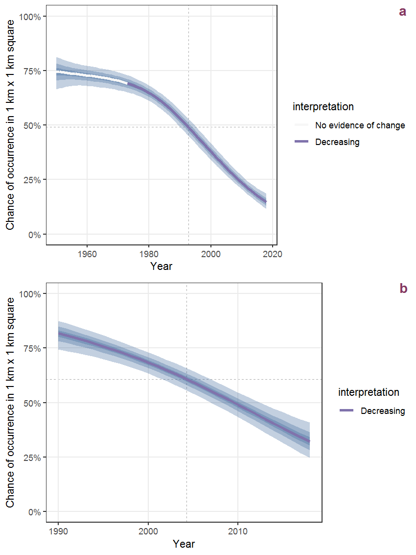
Figure F.64: Effect of year on the probability of Chrysanthemum segetum L. presence in 1 km x 1 km squares where the species has been observed at least once. The fitted line shows the sum of the overall mean (the intercept), a conditional effect of list-length equal to 130 and the year-smoother. The vertical dashed lines indicate the year(s) where the year-smoother is zero. The 95% confidence band is shown in grey (including the variability around the intercept and the smoother). a: 1950 - 2018, b: 1990 - 2018.
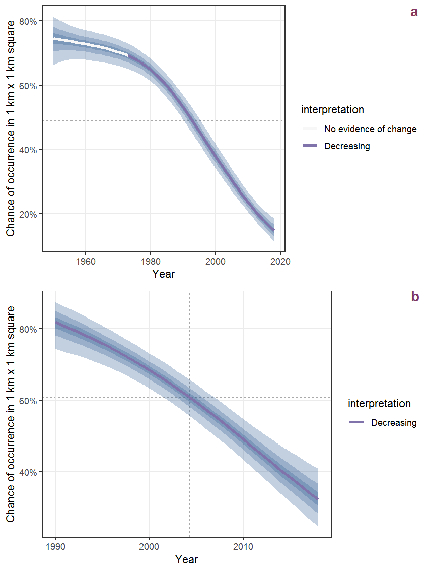
Figure F.65: The same as F.64, but the vertical axis is scaled to the range of the predicted values such that relative changes can be seen more easily. a: 1950 - 2018, b: 1990 - 2018.
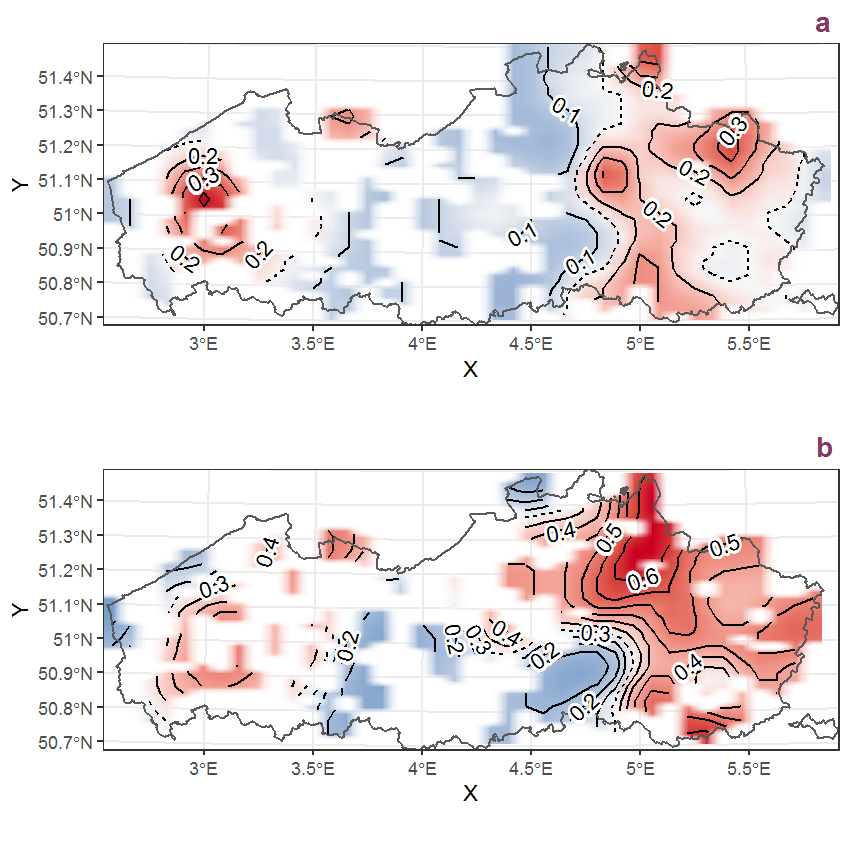
Figure F.66: Visualisation of the spatial smooth effect on the probability of Chrysanthemum segetum L. presence in 1 km x 1 km squares where the species has been observed at least once. The probabilities (values on the contour lines) are conditional on the final year of observation and a list-length equal to 130. The dashed contour line demarcates zones where the species is expected to be more prevalent (red shades) from zones where the species is less prevalent (blue shades). a: 1950 - 2018, b: 1990 - 2018.
F.23 Cichorium intybus L.
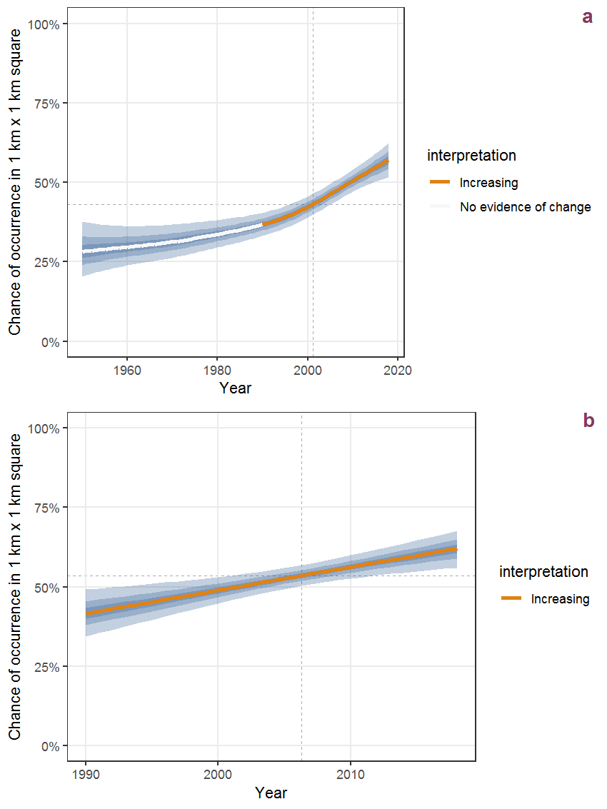
Figure F.67: Effect of year on the probability of Cichorium intybus L. presence in 1 km x 1 km squares where the species has been observed at least once. The fitted line shows the sum of the overall mean (the intercept), a conditional effect of list-length equal to 130 and the year-smoother. The vertical dashed lines indicate the year(s) where the year-smoother is zero. The 95% confidence band is shown in grey (including the variability around the intercept and the smoother). a: 1950 - 2018, b: 1990 - 2018.
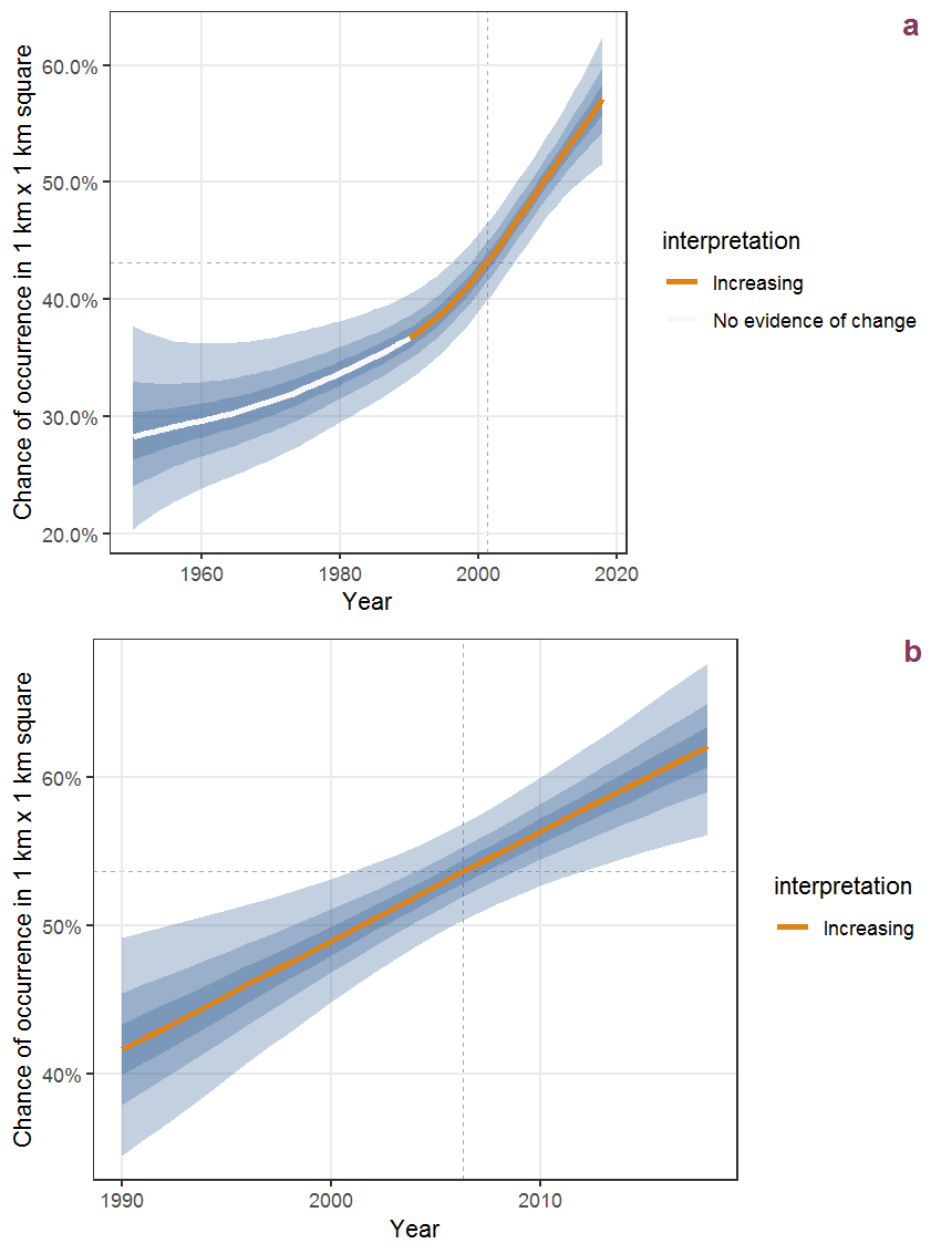
Figure F.68: The same as F.67, but the vertical axis is scaled to the range of the predicted values such that relative changes can be seen more easily. a: 1950 - 2018, b: 1990 - 2018.
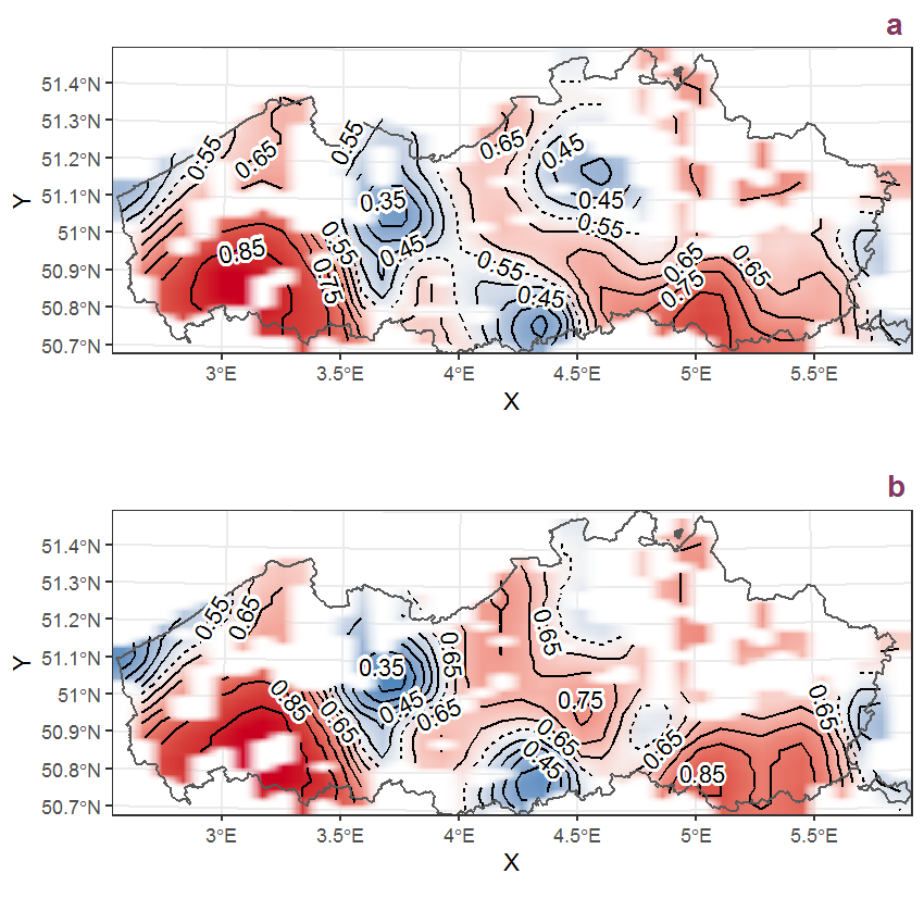
Figure F.69: Visualisation of the spatial smooth effect on the probability of Cichorium intybus L. presence in 1 km x 1 km squares where the species has been observed at least once. The probabilities (values on the contour lines) are conditional on the final year of observation and a list-length equal to 130. The dashed contour line demarcates zones where the species is expected to be more prevalent (red shades) from zones where the species is less prevalent (blue shades). a: 1950 - 2018, b: 1990 - 2018.
F.24 Circaea lutetiana L.
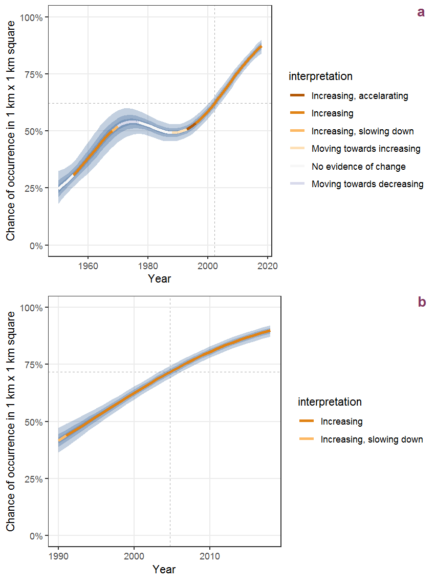
Figure F.70: Effect of year on the probability of Circaea lutetiana L. presence in 1 km x 1 km squares where the species has been observed at least once. The fitted line shows the sum of the overall mean (the intercept), a conditional effect of list-length equal to 130 and the year-smoother. The vertical dashed lines indicate the year(s) where the year-smoother is zero. The 95% confidence band is shown in grey (including the variability around the intercept and the smoother). a: 1950 - 2018, b: 1990 - 2018.
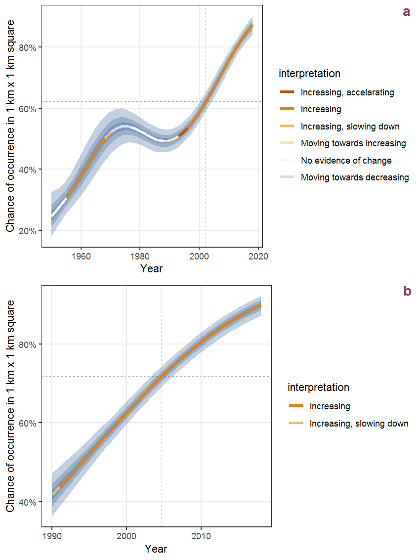
Figure F.71: The same as F.70, but the vertical axis is scaled to the range of the predicted values such that relative changes can be seen more easily. a: 1950 - 2018, b: 1990 - 2018.
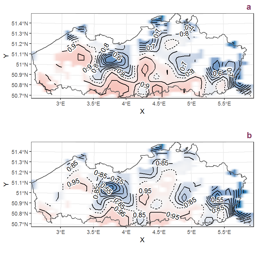
Figure F.72: Visualisation of the spatial smooth effect on the probability of Circaea lutetiana L. presence in 1 km x 1 km squares where the species has been observed at least once. The probabilities (values on the contour lines) are conditional on the final year of observation and a list-length equal to 130. The dashed contour line demarcates zones where the species is expected to be more prevalent (red shades) from zones where the species is less prevalent (blue shades). a: 1950 - 2018, b: 1990 - 2018.
F.25 Cirsium arvense (L.) Scop.
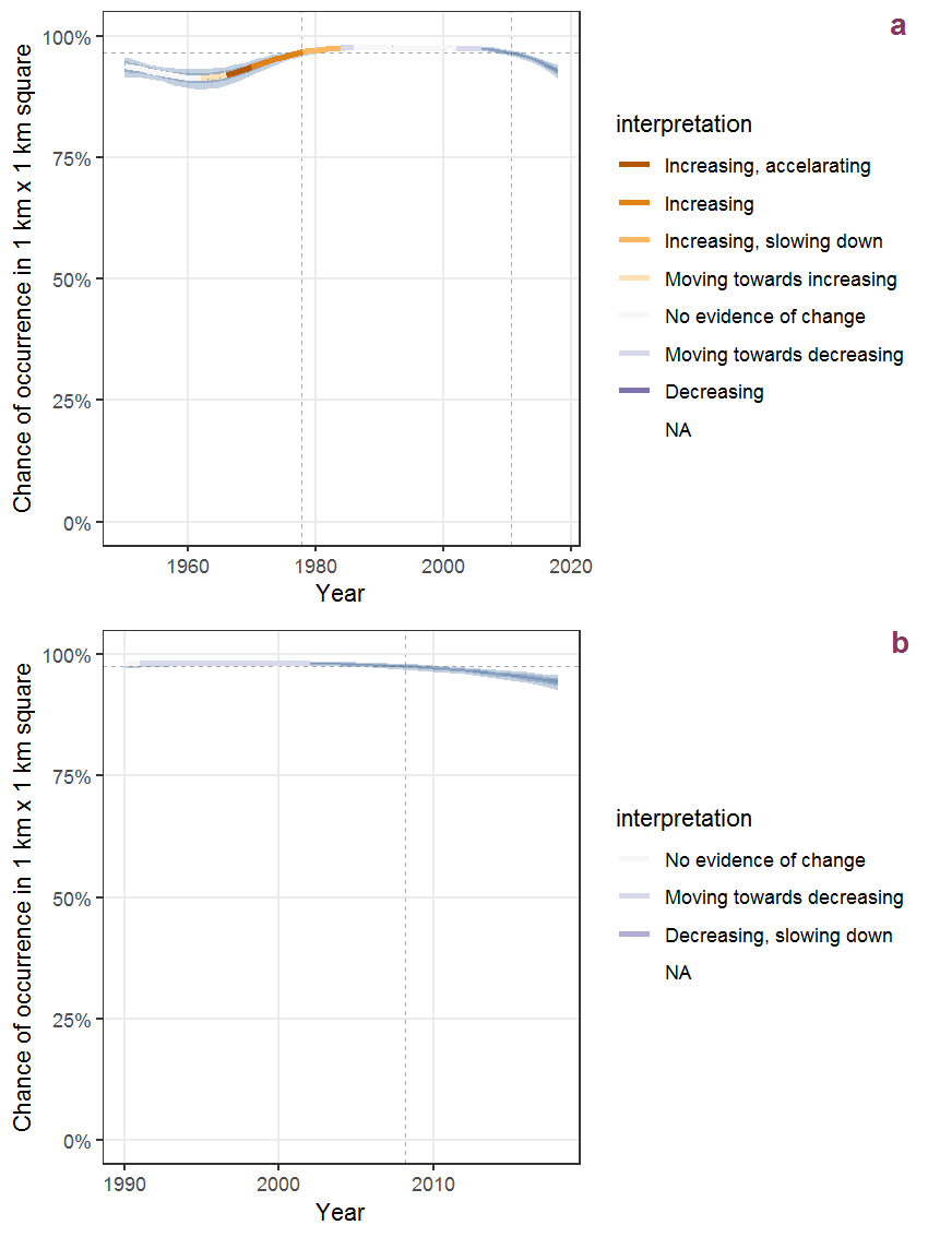
Figure F.73: Effect of year on the probability of Cirsium arvense (L.) Scop. presence in 1 km x 1 km squares where the species has been observed at least once. The fitted line shows the sum of the overall mean (the intercept), a conditional effect of list-length equal to 130 and the year-smoother. The vertical dashed lines indicate the year(s) where the year-smoother is zero. The 95% confidence band is shown in grey (including the variability around the intercept and the smoother). a: 1950 - 2018, b: 1990 - 2018.
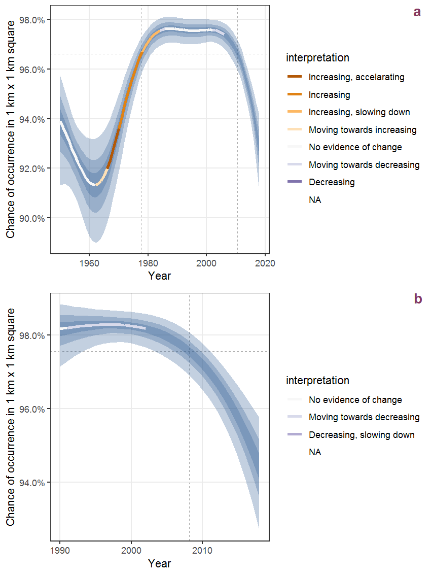
Figure F.74: The same as F.73, but the vertical axis is scaled to the range of the predicted values such that relative changes can be seen more easily. a: 1950 - 2018, b: 1990 - 2018.
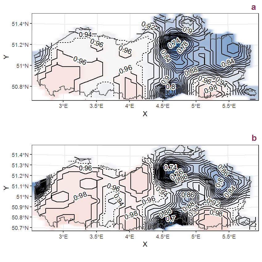
Figure F.75: Visualisation of the spatial smooth effect on the probability of Cirsium arvense (L.) Scop. presence in 1 km x 1 km squares where the species has been observed at least once. The probabilities (values on the contour lines) are conditional on the final year of observation and a list-length equal to 130. The dashed contour line demarcates zones where the species is expected to be more prevalent (red shades) from zones where the species is less prevalent (blue shades). a: 1950 - 2018, b: 1990 - 2018.
F.26 Cirsium oleraceum (L.) Scop.
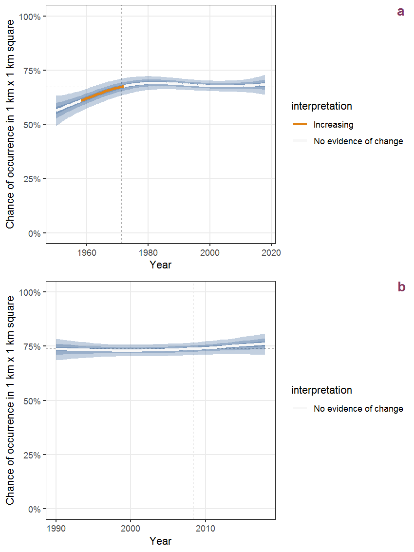
Figure F.76: Effect of year on the probability of Cirsium oleraceum (L.) Scop. presence in 1 km x 1 km squares where the species has been observed at least once. The fitted line shows the sum of the overall mean (the intercept), a conditional effect of list-length equal to 130 and the year-smoother. The vertical dashed lines indicate the year(s) where the year-smoother is zero. The 95% confidence band is shown in grey (including the variability around the intercept and the smoother). a: 1950 - 2018, b: 1990 - 2018.
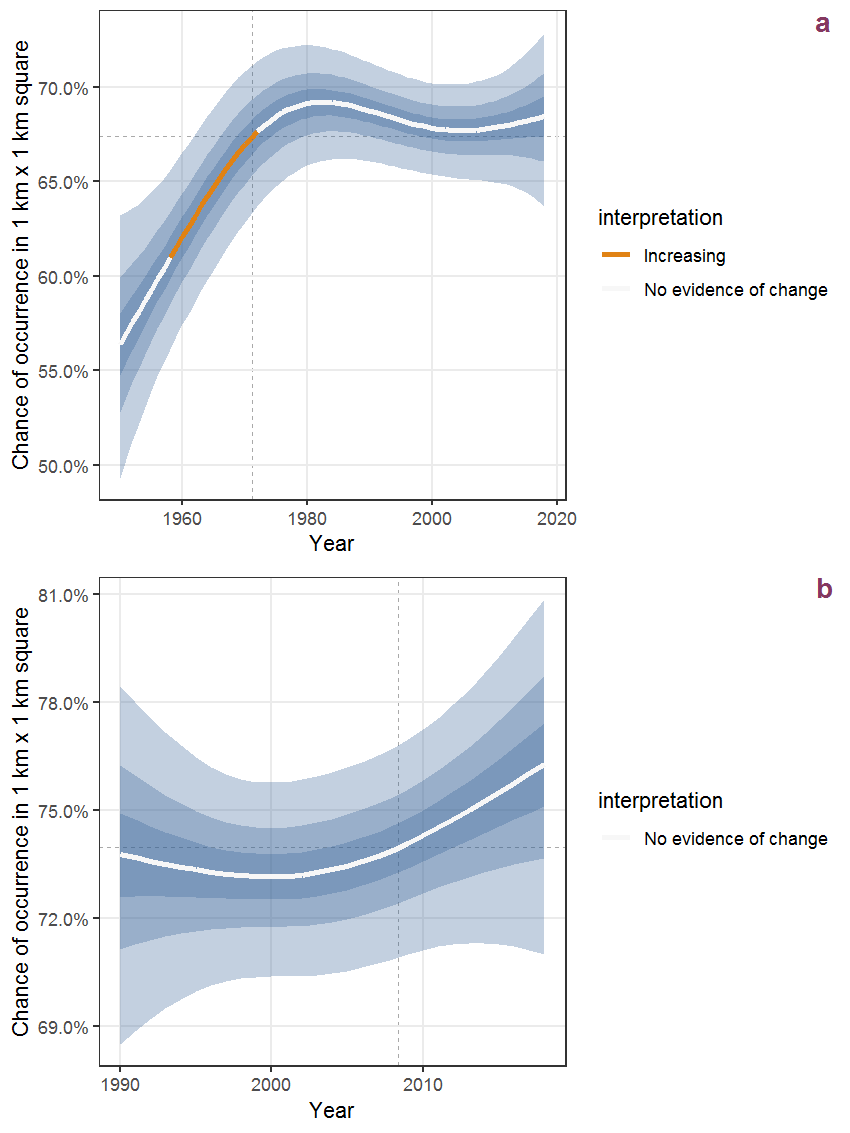
Figure F.77: The same as F.76, but the vertical axis is scaled to the range of the predicted values such that relative changes can be seen more easily. a: 1950 - 2018, b: 1990 - 2018.
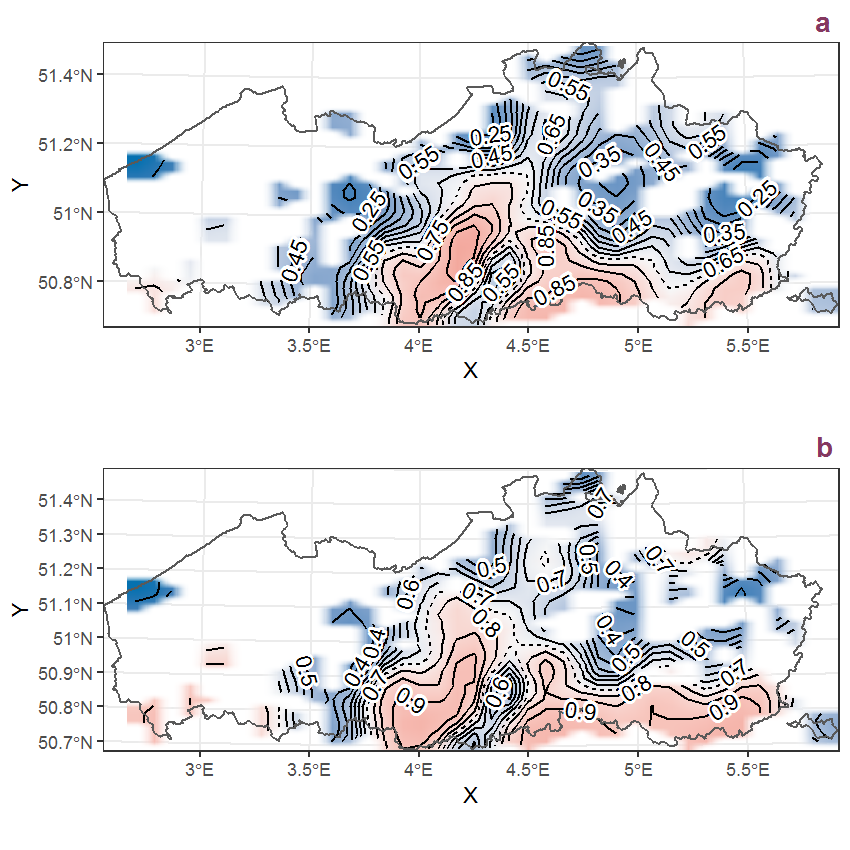
Figure F.78: Visualisation of the spatial smooth effect on the probability of Cirsium oleraceum (L.) Scop. presence in 1 km x 1 km squares where the species has been observed at least once. The probabilities (values on the contour lines) are conditional on the final year of observation and a list-length equal to 130. The dashed contour line demarcates zones where the species is expected to be more prevalent (red shades) from zones where the species is less prevalent (blue shades). a: 1950 - 2018, b: 1990 - 2018.
F.27 Cirsium palustre (L.) Scop.
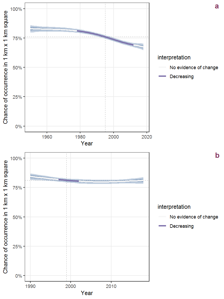
Figure F.79: Effect of year on the probability of Cirsium palustre (L.) Scop. presence in 1 km x 1 km squares where the species has been observed at least once. The fitted line shows the sum of the overall mean (the intercept), a conditional effect of list-length equal to 130 and the year-smoother. The vertical dashed lines indicate the year(s) where the year-smoother is zero. The 95% confidence band is shown in grey (including the variability around the intercept and the smoother). a: 1950 - 2018, b: 1990 - 2018.

Figure F.80: The same as F.79, but the vertical axis is scaled to the range of the predicted values such that relative changes can be seen more easily. a: 1950 - 2018, b: 1990 - 2018.
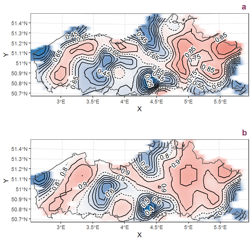
Figure F.81: Visualisation of the spatial smooth effect on the probability of Cirsium palustre (L.) Scop. presence in 1 km x 1 km squares where the species has been observed at least once. The probabilities (values on the contour lines) are conditional on the final year of observation and a list-length equal to 130. The dashed contour line demarcates zones where the species is expected to be more prevalent (red shades) from zones where the species is less prevalent (blue shades). a: 1950 - 2018, b: 1990 - 2018.
F.28 Cirsium vulgare (Savi) Ten.
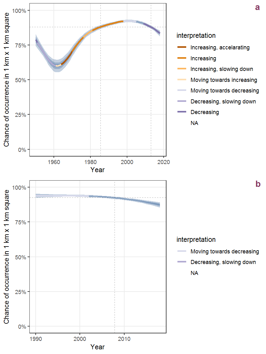
Figure F.82: Effect of year on the probability of Cirsium vulgare (Savi) Ten. presence in 1 km x 1 km squares where the species has been observed at least once. The fitted line shows the sum of the overall mean (the intercept), a conditional effect of list-length equal to 130 and the year-smoother. The vertical dashed lines indicate the year(s) where the year-smoother is zero. The 95% confidence band is shown in grey (including the variability around the intercept and the smoother). a: 1950 - 2018, b: 1990 - 2018.
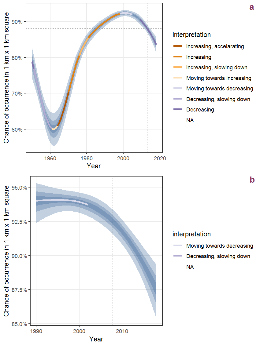
Figure F.83: The same as F.82, but the vertical axis is scaled to the range of the predicted values such that relative changes can be seen more easily. a: 1950 - 2018, b: 1990 - 2018.
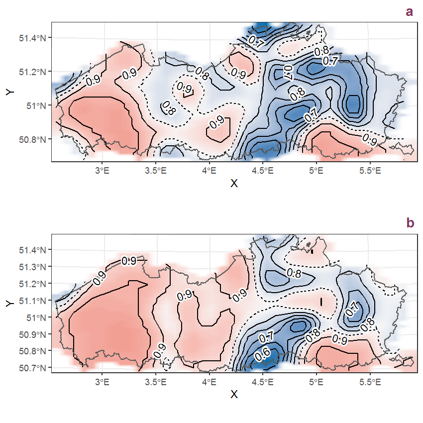
Figure F.84: Visualisation of the spatial smooth effect on the probability of Cirsium vulgare (Savi) Ten. presence in 1 km x 1 km squares where the species has been observed at least once. The probabilities (values on the contour lines) are conditional on the final year of observation and a list-length equal to 130. The dashed contour line demarcates zones where the species is expected to be more prevalent (red shades) from zones where the species is less prevalent (blue shades). a: 1950 - 2018, b: 1990 - 2018.
F.29 Claytonia perfoliata Donn ex Willd.
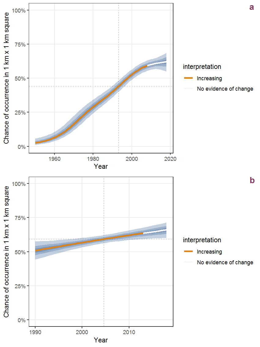
Figure F.85: Effect of year on the probability of Claytonia perfoliata Donn ex Willd. presence in 1 km x 1 km squares where the species has been observed at least once. The fitted line shows the sum of the overall mean (the intercept), a conditional effect of list-length equal to 130 and the year-smoother. The vertical dashed lines indicate the year(s) where the year-smoother is zero. The 95% confidence band is shown in grey (including the variability around the intercept and the smoother). a: 1950 - 2018, b: 1990 - 2018.
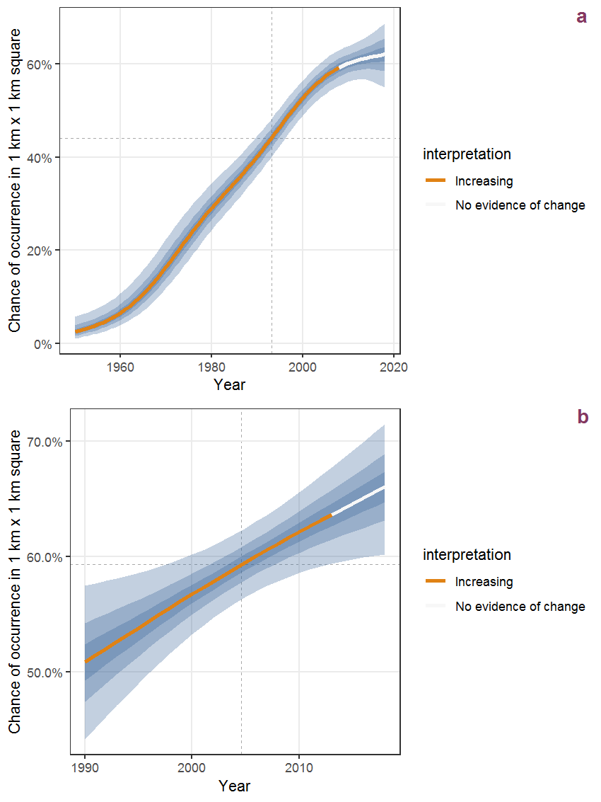
Figure F.86: The same as F.85, but the vertical axis is scaled to the range of the predicted values such that relative changes can be seen more easily. a: 1950 - 2018, b: 1990 - 2018.
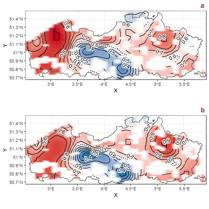
Figure F.87: Visualisation of the spatial smooth effect on the probability of Claytonia perfoliata Donn ex Willd. presence in 1 km x 1 km squares where the species has been observed at least once. The probabilities (values on the contour lines) are conditional on the final year of observation and a list-length equal to 130. The dashed contour line demarcates zones where the species is expected to be more prevalent (red shades) from zones where the species is less prevalent (blue shades). a: 1950 - 2018, b: 1990 - 2018.
F.30 Clematis vitalba L.
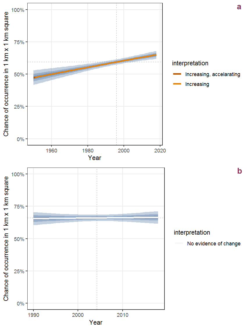
Figure F.88: Effect of year on the probability of Clematis vitalba L. presence in 1 km x 1 km squares where the species has been observed at least once. The fitted line shows the sum of the overall mean (the intercept), a conditional effect of list-length equal to 130 and the year-smoother. The vertical dashed lines indicate the year(s) where the year-smoother is zero. The 95% confidence band is shown in grey (including the variability around the intercept and the smoother). a: 1950 - 2018, b: 1990 - 2018.
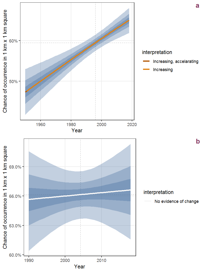
Figure F.89: The same as F.88, but the vertical axis is scaled to the range of the predicted values such that relative changes can be seen more easily. a: 1950 - 2018, b: 1990 - 2018.
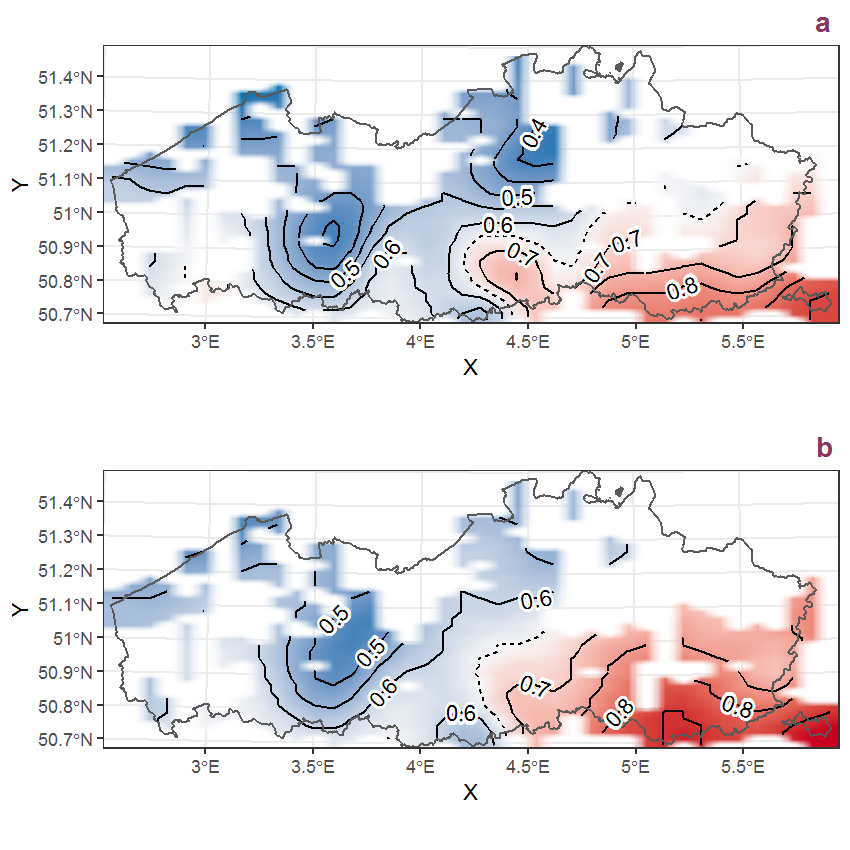
Figure F.90: Visualisation of the spatial smooth effect on the probability of Clematis vitalba L. presence in 1 km x 1 km squares where the species has been observed at least once. The probabilities (values on the contour lines) are conditional on the final year of observation and a list-length equal to 130. The dashed contour line demarcates zones where the species is expected to be more prevalent (red shades) from zones where the species is less prevalent (blue shades). a: 1950 - 2018, b: 1990 - 2018.
F.31 Conium maculatum L.
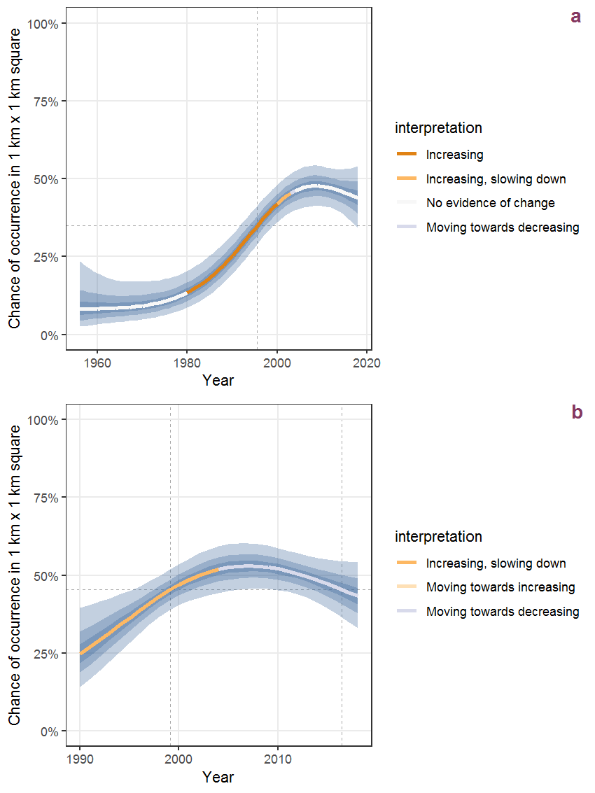
Figure F.91: Effect of year on the probability of Conium maculatum L. presence in 1 km x 1 km squares where the species has been observed at least once. The fitted line shows the sum of the overall mean (the intercept), a conditional effect of list-length equal to 130 and the year-smoother. The vertical dashed lines indicate the year(s) where the year-smoother is zero. The 95% confidence band is shown in grey (including the variability around the intercept and the smoother). a: 1950 - 2018, b: 1990 - 2018.
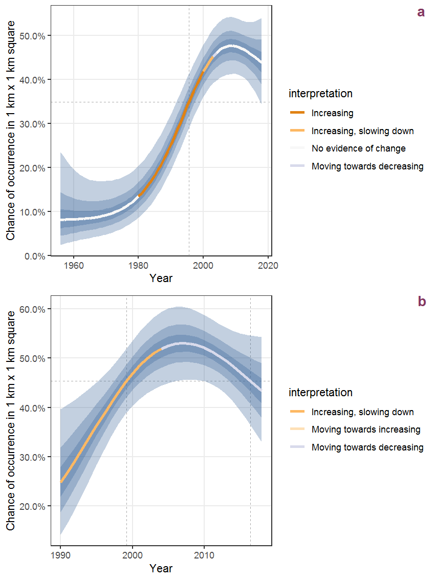
Figure F.92: The same as F.91, but the vertical axis is scaled to the range of the predicted values such that relative changes can be seen more easily. a: 1950 - 2018, b: 1990 - 2018.
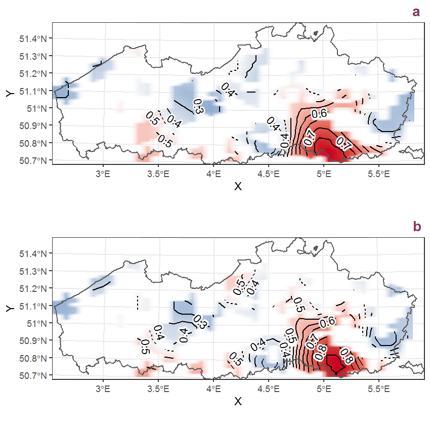
Figure F.93: Visualisation of the spatial smooth effect on the probability of Conium maculatum L. presence in 1 km x 1 km squares where the species has been observed at least once. The probabilities (values on the contour lines) are conditional on the final year of observation and a list-length equal to 130. The dashed contour line demarcates zones where the species is expected to be more prevalent (red shades) from zones where the species is less prevalent (blue shades). a: 1950 - 2018, b: 1990 - 2018.
F.32 Convallaria majalis L.
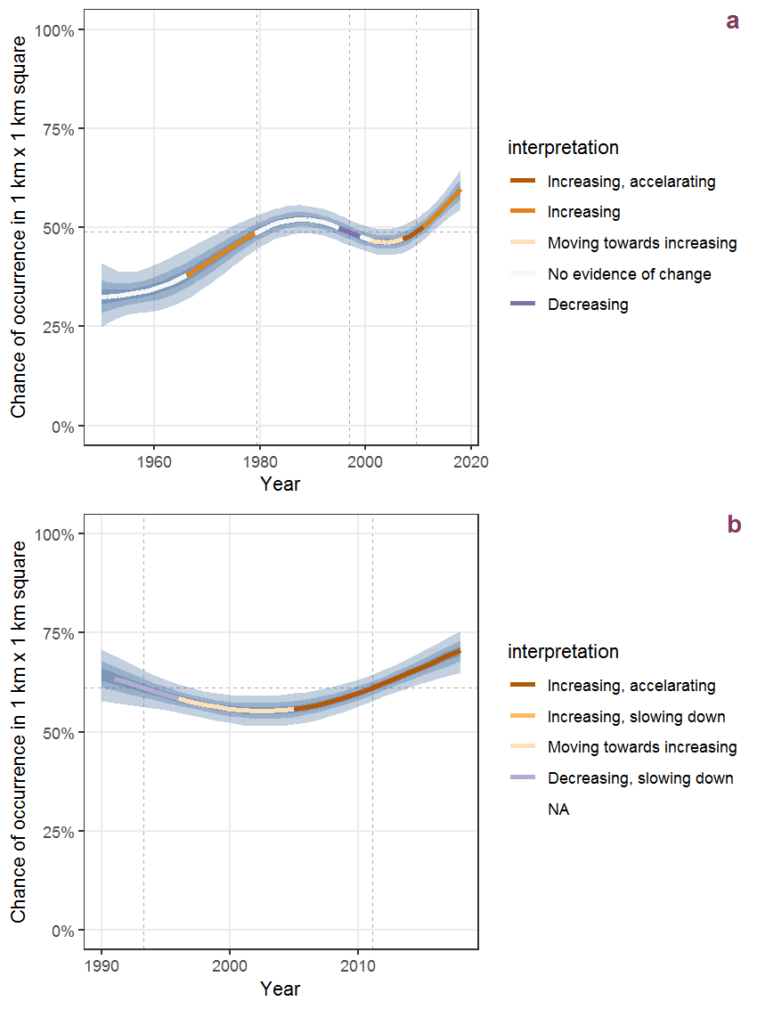
Figure F.94: Effect of year on the probability of Convallaria majalis L. presence in 1 km x 1 km squares where the species has been observed at least once. The fitted line shows the sum of the overall mean (the intercept), a conditional effect of list-length equal to 130 and the year-smoother. The vertical dashed lines indicate the year(s) where the year-smoother is zero. The 95% confidence band is shown in grey (including the variability around the intercept and the smoother). a: 1950 - 2018, b: 1990 - 2018.
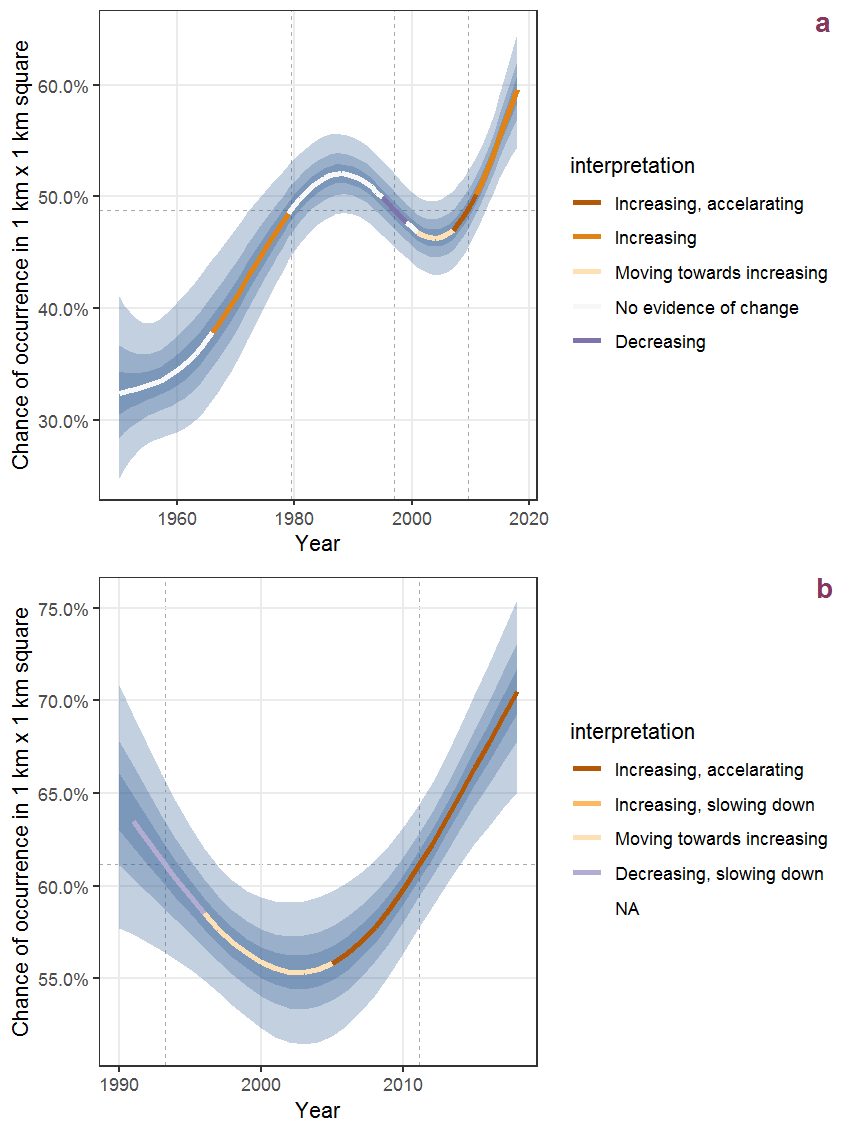
Figure F.95: The same as F.94, but the vertical axis is scaled to the range of the predicted values such that relative changes can be seen more easily. a: 1950 - 2018, b: 1990 - 2018.
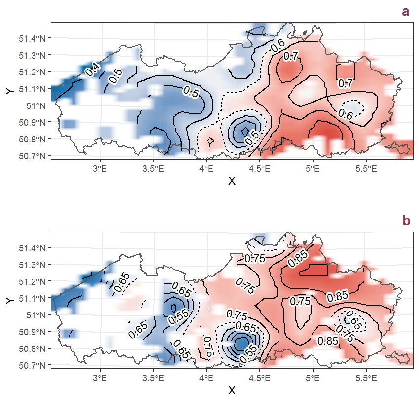
Figure F.96: Visualisation of the spatial smooth effect on the probability of Convallaria majalis L. presence in 1 km x 1 km squares where the species has been observed at least once. The probabilities (values on the contour lines) are conditional on the final year of observation and a list-length equal to 130. The dashed contour line demarcates zones where the species is expected to be more prevalent (red shades) from zones where the species is less prevalent (blue shades). a: 1950 - 2018, b: 1990 - 2018.