P Potamogeton natans L. - Raphanus raphanistrum L.
P.1 Potamogeton natans L.
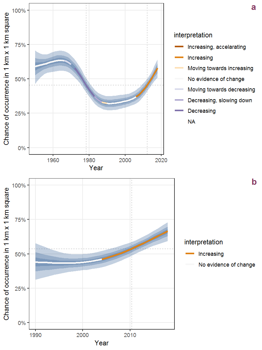
Figure P.1: Effect of year on the probability of Potamogeton natans L. presence in 1 km x 1 km squares where the species has been observed at least once. The fitted line shows the sum of the overall mean (the intercept), a conditional effect of list-length equal to 130 and the year-smoother. The vertical dashed lines indicate the year(s) where the year-smoother is zero. The 95% confidence band is shown in grey (including the variability around the intercept and the smoother). a: 1950 - 2018, b: 1990 - 2018.
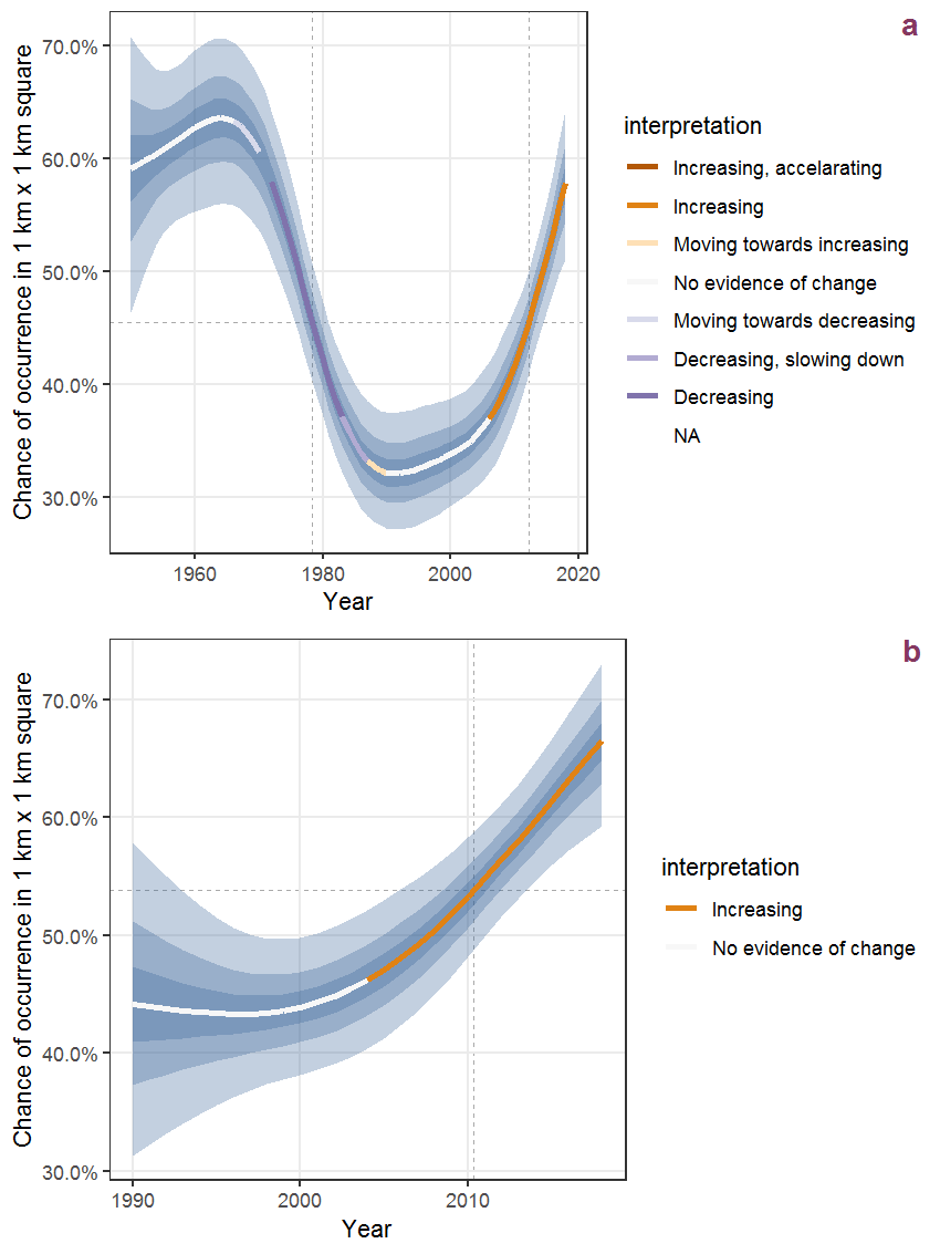
Figure P.2: The same as P.1, but the vertical axis is scaled to the range of the predicted values such that relative changes can be seen more easily. a: 1950 - 2018, b: 1990 - 2018.
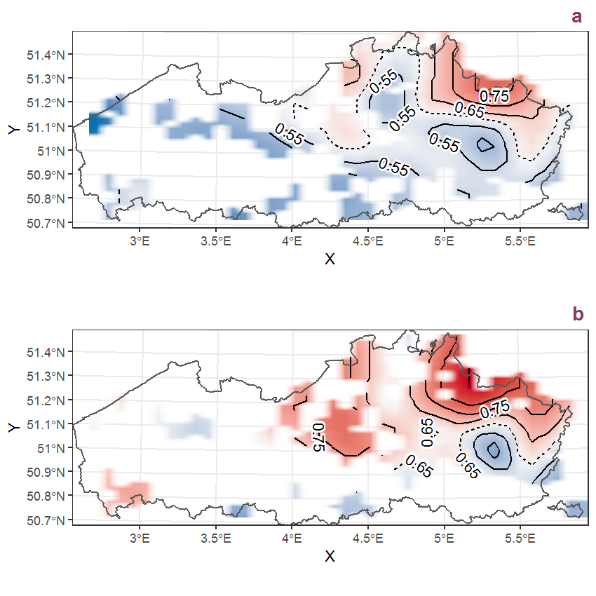
Figure P.3: Visualisation of the spatial smooth effect on the probability of Potamogeton natans L. presence in 1 km x 1 km squares where the species has been observed at least once. The probabilities (values on the contour lines) are conditional on the final year of observation and a list-length equal to 130. The dashed contour line demarcates zones where the species is expected to be more prevalent (red shades) from zones where the species is less prevalent (blue shades). a: 1950 - 2018, b: 1990 - 2018.
P.2 Potamogeton pectinatus L.
Figure P.4: Effect of year on the probability of Potamogeton pectinatus L. presence in 1 km x 1 km squares where the species has been observed at least once. The fitted line shows the sum of the overall mean (the intercept), a conditional effect of list-length equal to 130 and the year-smoother. The vertical dashed lines indicate the year(s) where the year-smoother is zero. The 95% confidence band is shown in grey (including the variability around the intercept and the smoother). a: 1950 - 2018, b: 1990 - 2018.
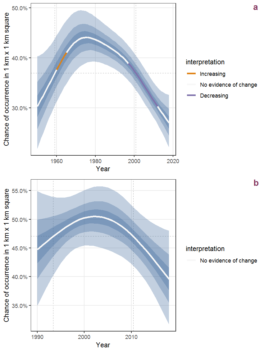
Figure P.5: The same as P.4, but the vertical axis is scaled to the range of the predicted values such that relative changes can be seen more easily. a: 1950 - 2018, b: 1990 - 2018.
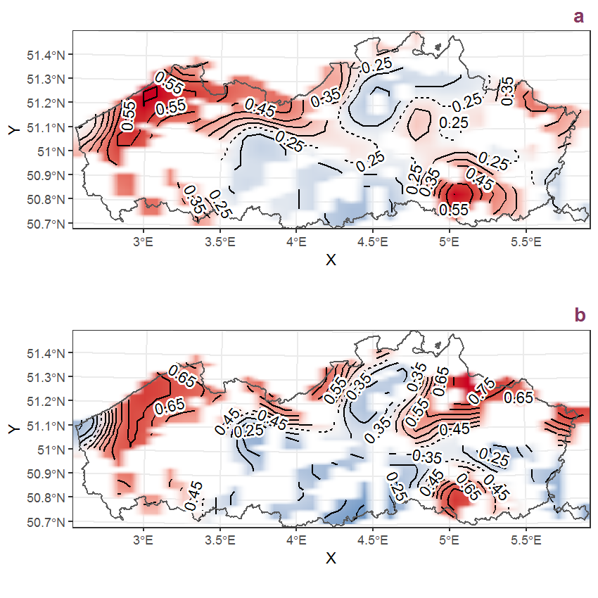
Figure P.6: Visualisation of the spatial smooth effect on the probability of Potamogeton pectinatus L. presence in 1 km x 1 km squares where the species has been observed at least once. The probabilities (values on the contour lines) are conditional on the final year of observation and a list-length equal to 130. The dashed contour line demarcates zones where the species is expected to be more prevalent (red shades) from zones where the species is less prevalent (blue shades). a: 1950 - 2018, b: 1990 - 2018.
P.3 Potamogeton polygonifolius Pourr.
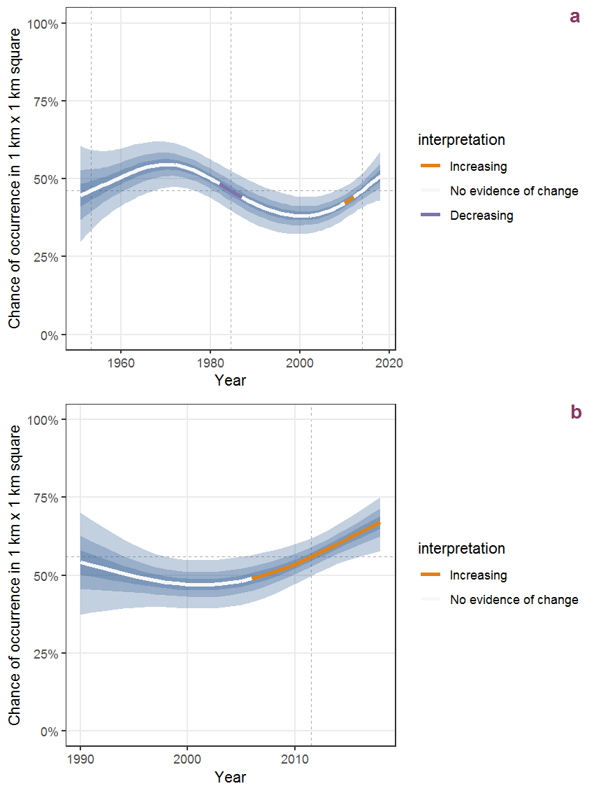
Figure P.7: Effect of year on the probability of Potamogeton polygonifolius Pourr. presence in 1 km x 1 km squares where the species has been observed at least once. The fitted line shows the sum of the overall mean (the intercept), a conditional effect of list-length equal to 130 and the year-smoother. The vertical dashed lines indicate the year(s) where the year-smoother is zero. The 95% confidence band is shown in grey (including the variability around the intercept and the smoother). a: 1950 - 2018, b: 1990 - 2018.
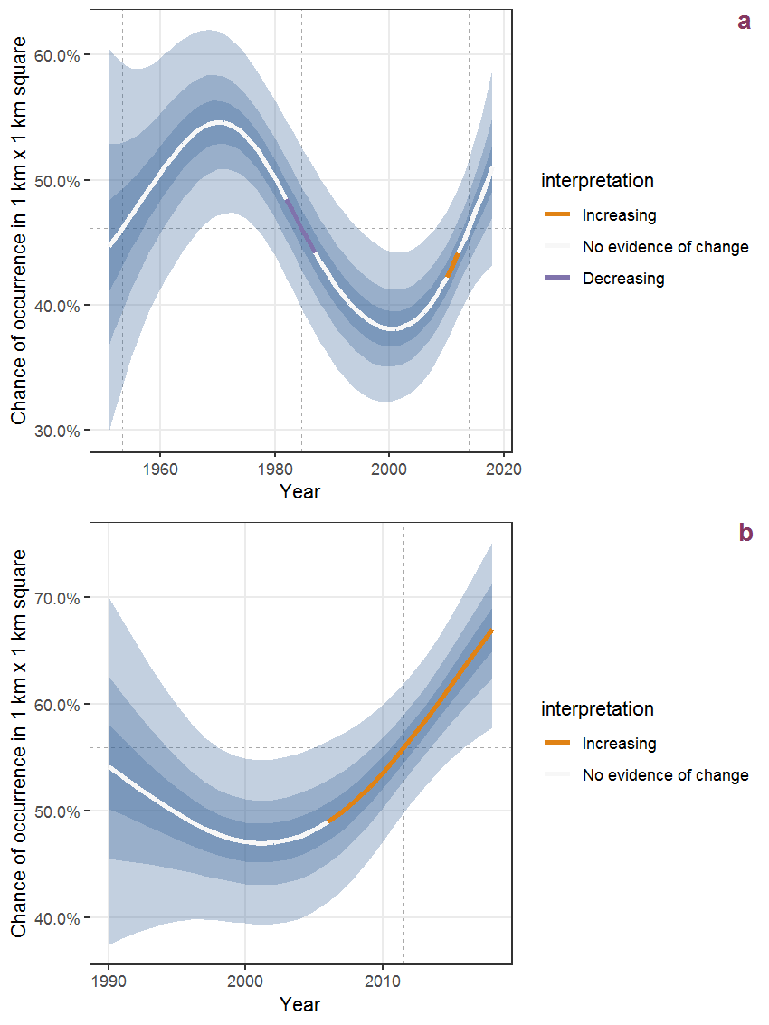
Figure P.8: The same as P.7, but the vertical axis is scaled to the range of the predicted values such that relative changes can be seen more easily. a: 1950 - 2018, b: 1990 - 2018.
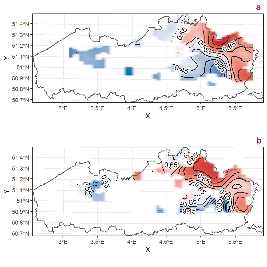
Figure P.9: Visualisation of the spatial smooth effect on the probability of Potamogeton polygonifolius Pourr. presence in 1 km x 1 km squares where the species has been observed at least once. The probabilities (values on the contour lines) are conditional on the final year of observation and a list-length equal to 130. The dashed contour line demarcates zones where the species is expected to be more prevalent (red shades) from zones where the species is less prevalent (blue shades). a: 1950 - 2018, b: 1990 - 2018.
P.4 Potentilla anglica Laichard.
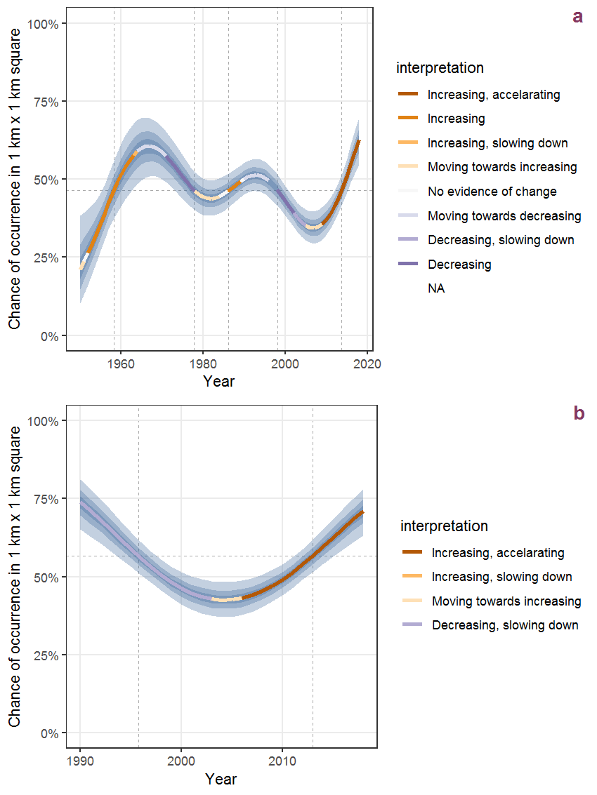
Figure P.10: Effect of year on the probability of Potentilla anglica Laichard. presence in 1 km x 1 km squares where the species has been observed at least once. The fitted line shows the sum of the overall mean (the intercept), a conditional effect of list-length equal to 130 and the year-smoother. The vertical dashed lines indicate the year(s) where the year-smoother is zero. The 95% confidence band is shown in grey (including the variability around the intercept and the smoother). a: 1950 - 2018, b: 1990 - 2018.
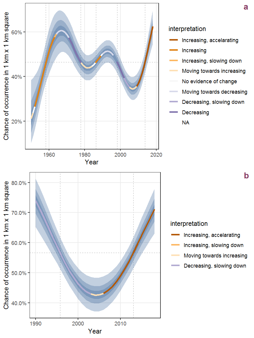
Figure P.11: The same as P.10, but the vertical axis is scaled to the range of the predicted values such that relative changes can be seen more easily. a: 1950 - 2018, b: 1990 - 2018.
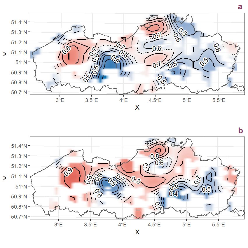
Figure P.12: Visualisation of the spatial smooth effect on the probability of Potentilla anglica Laichard. presence in 1 km x 1 km squares where the species has been observed at least once. The probabilities (values on the contour lines) are conditional on the final year of observation and a list-length equal to 130. The dashed contour line demarcates zones where the species is expected to be more prevalent (red shades) from zones where the species is less prevalent (blue shades). a: 1950 - 2018, b: 1990 - 2018.
P.5 Potentilla anserina L.
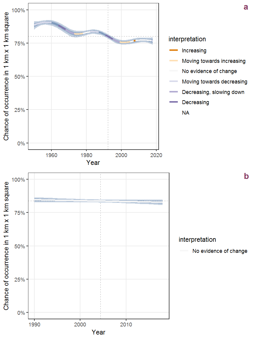
Figure P.13: Effect of year on the probability of Potentilla anserina L. presence in 1 km x 1 km squares where the species has been observed at least once. The fitted line shows the sum of the overall mean (the intercept), a conditional effect of list-length equal to 130 and the year-smoother. The vertical dashed lines indicate the year(s) where the year-smoother is zero. The 95% confidence band is shown in grey (including the variability around the intercept and the smoother). a: 1950 - 2018, b: 1990 - 2018.
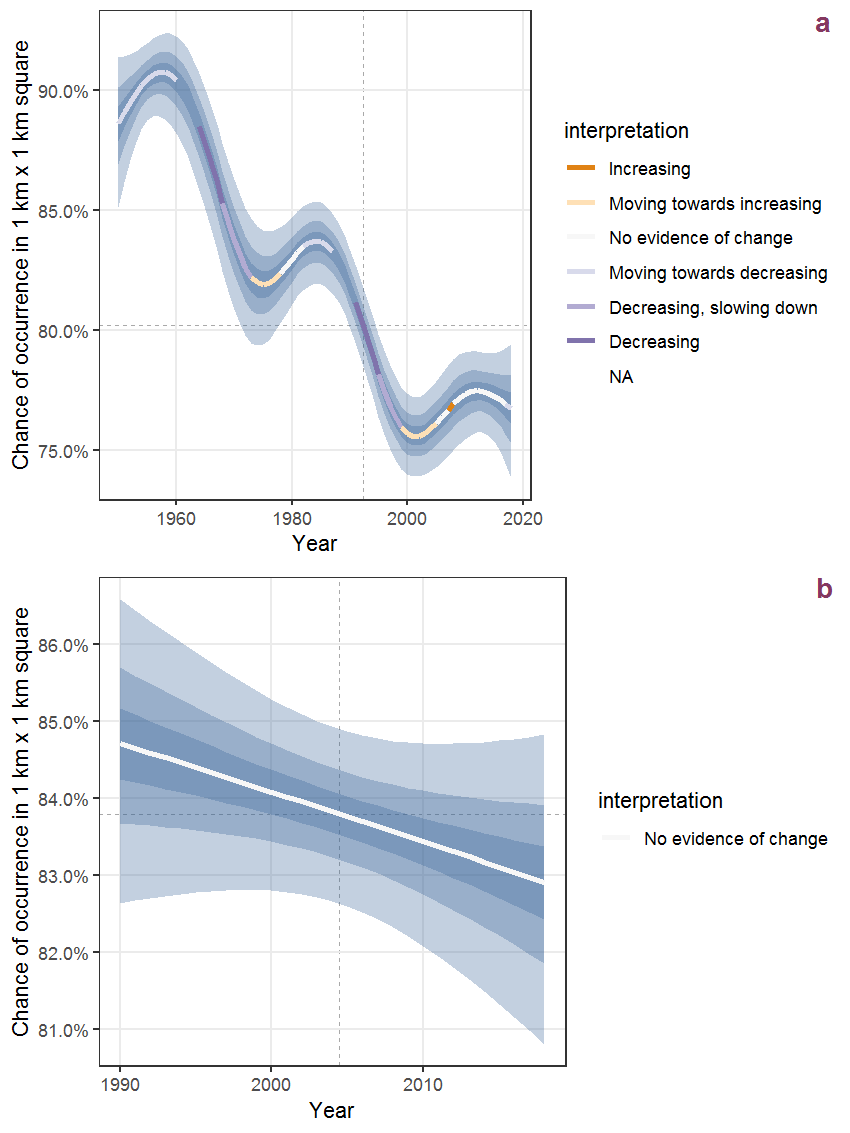
Figure P.14: The same as P.13, but the vertical axis is scaled to the range of the predicted values such that relative changes can be seen more easily. a: 1950 - 2018, b: 1990 - 2018.
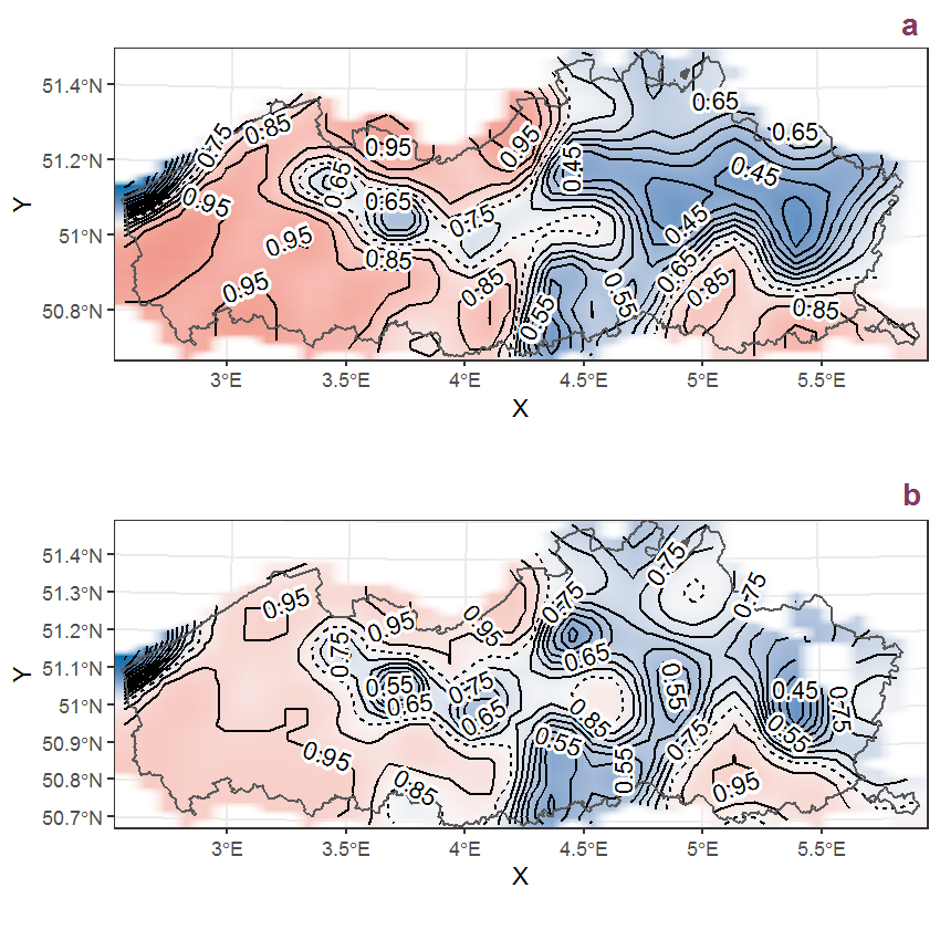
Figure P.15: Visualisation of the spatial smooth effect on the probability of Potentilla anserina L. presence in 1 km x 1 km squares where the species has been observed at least once. The probabilities (values on the contour lines) are conditional on the final year of observation and a list-length equal to 130. The dashed contour line demarcates zones where the species is expected to be more prevalent (red shades) from zones where the species is less prevalent (blue shades). a: 1950 - 2018, b: 1990 - 2018.
P.6 Potentilla erecta (L.) Räuschel
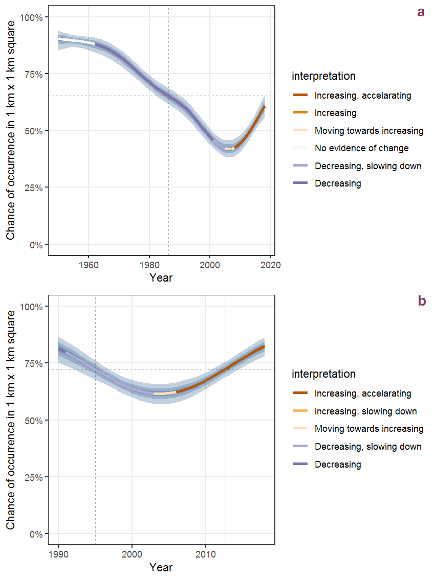
Figure P.16: Effect of year on the probability of Potentilla erecta (L.) Räuschel presence in 1 km x 1 km squares where the species has been observed at least once. The fitted line shows the sum of the overall mean (the intercept), a conditional effect of list-length equal to 130 and the year-smoother. The vertical dashed lines indicate the year(s) where the year-smoother is zero. The 95% confidence band is shown in grey (including the variability around the intercept and the smoother). a: 1950 - 2018, b: 1990 - 2018.
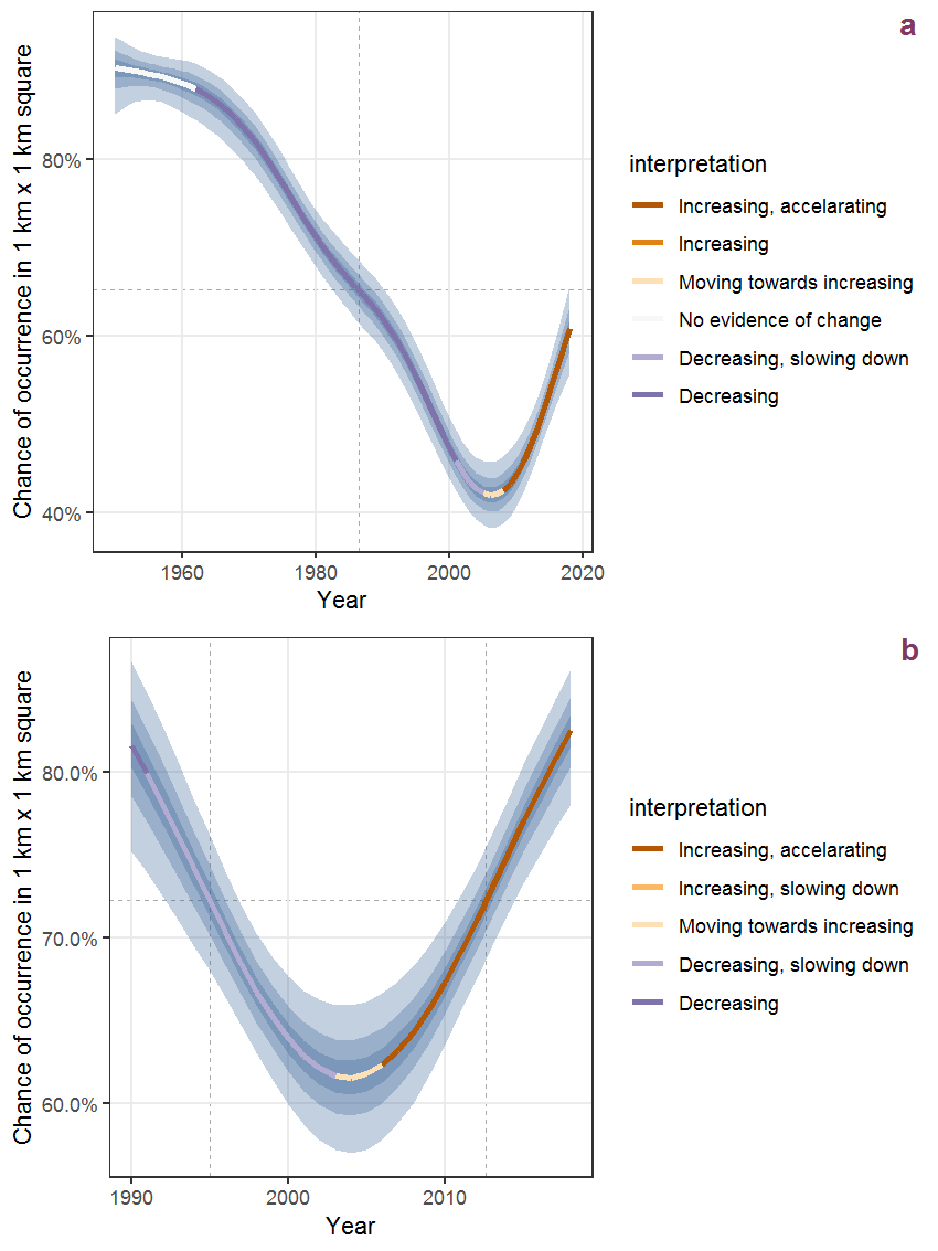
Figure P.17: The same as P.16, but the vertical axis is scaled to the range of the predicted values such that relative changes can be seen more easily. a: 1950 - 2018, b: 1990 - 2018.
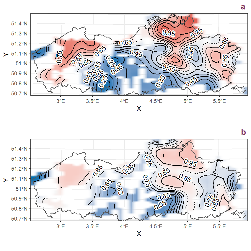
Figure P.18: Visualisation of the spatial smooth effect on the probability of Potentilla erecta (L.) Räuschel presence in 1 km x 1 km squares where the species has been observed at least once. The probabilities (values on the contour lines) are conditional on the final year of observation and a list-length equal to 130. The dashed contour line demarcates zones where the species is expected to be more prevalent (red shades) from zones where the species is less prevalent (blue shades). a: 1950 - 2018, b: 1990 - 2018.
P.7 Comarum palustre L.
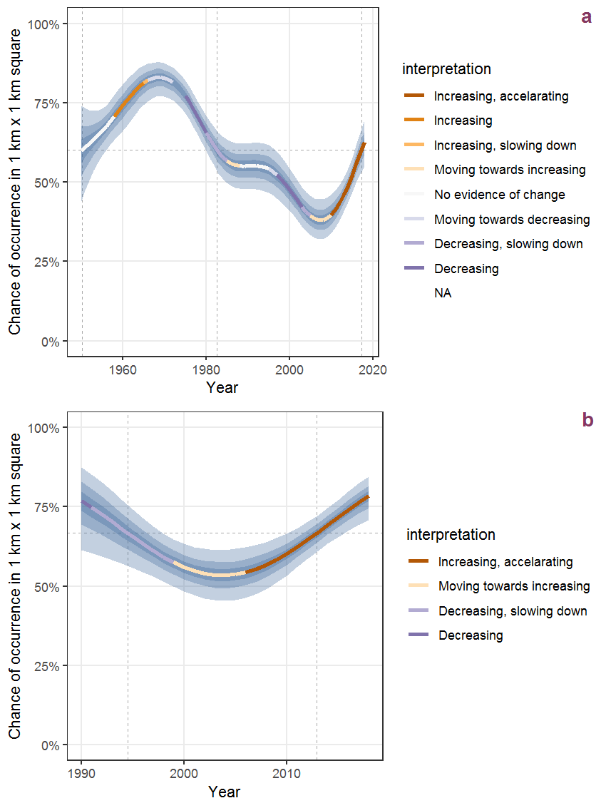
Figure P.19: Effect of year on the probability of Comarum palustre L. presence in 1 km x 1 km squares where the species has been observed at least once. The fitted line shows the sum of the overall mean (the intercept), a conditional effect of list-length equal to 130 and the year-smoother. The vertical dashed lines indicate the year(s) where the year-smoother is zero. The 95% confidence band is shown in grey (including the variability around the intercept and the smoother). a: 1950 - 2018, b: 1990 - 2018.
Figure P.20: The same as P.19, but the vertical axis is scaled to the range of the predicted values such that relative changes can be seen more easily. a: 1950 - 2018, b: 1990 - 2018.
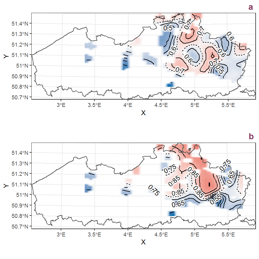
Figure P.21: Visualisation of the spatial smooth effect on the probability of Comarum palustre L. presence in 1 km x 1 km squares where the species has been observed at least once. The probabilities (values on the contour lines) are conditional on the final year of observation and a list-length equal to 130. The dashed contour line demarcates zones where the species is expected to be more prevalent (red shades) from zones where the species is less prevalent (blue shades). a: 1950 - 2018, b: 1990 - 2018.
P.8 Potentilla reptans L.
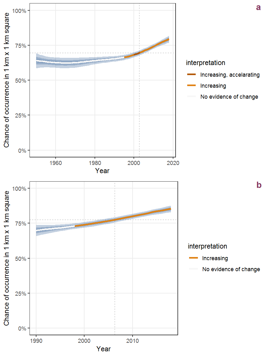
Figure P.22: Effect of year on the probability of Potentilla reptans L. presence in 1 km x 1 km squares where the species has been observed at least once. The fitted line shows the sum of the overall mean (the intercept), a conditional effect of list-length equal to 130 and the year-smoother. The vertical dashed lines indicate the year(s) where the year-smoother is zero. The 95% confidence band is shown in grey (including the variability around the intercept and the smoother). a: 1950 - 2018, b: 1990 - 2018.
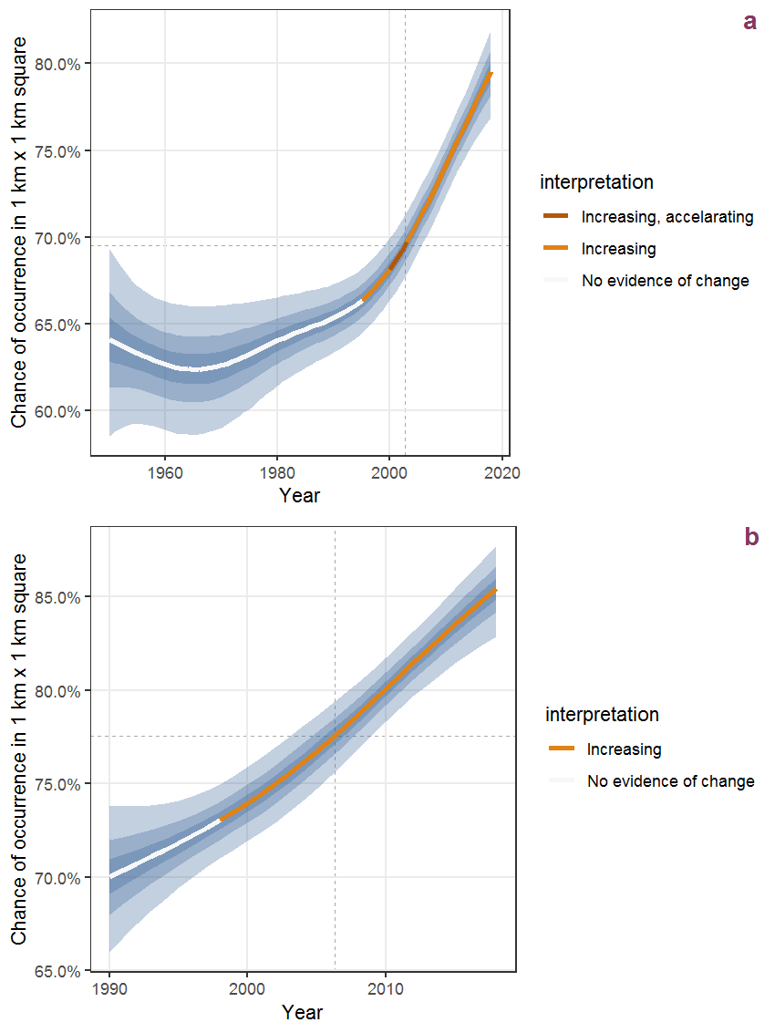
Figure P.23: The same as P.22, but the vertical axis is scaled to the range of the predicted values such that relative changes can be seen more easily. a: 1950 - 2018, b: 1990 - 2018.

Figure P.24: Visualisation of the spatial smooth effect on the probability of Potentilla reptans L. presence in 1 km x 1 km squares where the species has been observed at least once. The probabilities (values on the contour lines) are conditional on the final year of observation and a list-length equal to 130. The dashed contour line demarcates zones where the species is expected to be more prevalent (red shades) from zones where the species is less prevalent (blue shades). a: 1950 - 2018, b: 1990 - 2018.
P.9 Potentilla sterilis (L.) Garcke
Figure P.25: Effect of year on the probability of Potentilla sterilis (L.) Garcke presence in 1 km x 1 km squares where the species has been observed at least once. The fitted line shows the sum of the overall mean (the intercept), a conditional effect of list-length equal to 130 and the year-smoother. The vertical dashed lines indicate the year(s) where the year-smoother is zero. The 95% confidence band is shown in grey (including the variability around the intercept and the smoother). a: 1950 - 2018, b: 1990 - 2018.
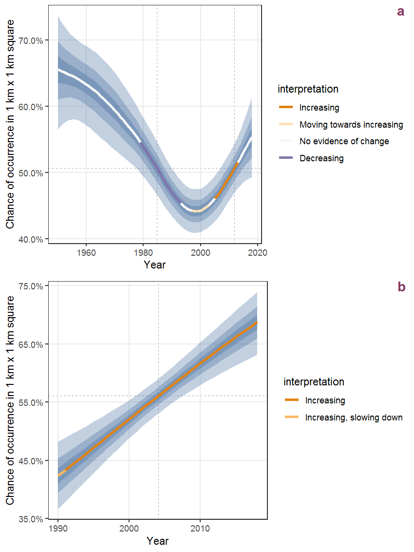
Figure P.26: The same as P.25, but the vertical axis is scaled to the range of the predicted values such that relative changes can be seen more easily. a: 1950 - 2018, b: 1990 - 2018.
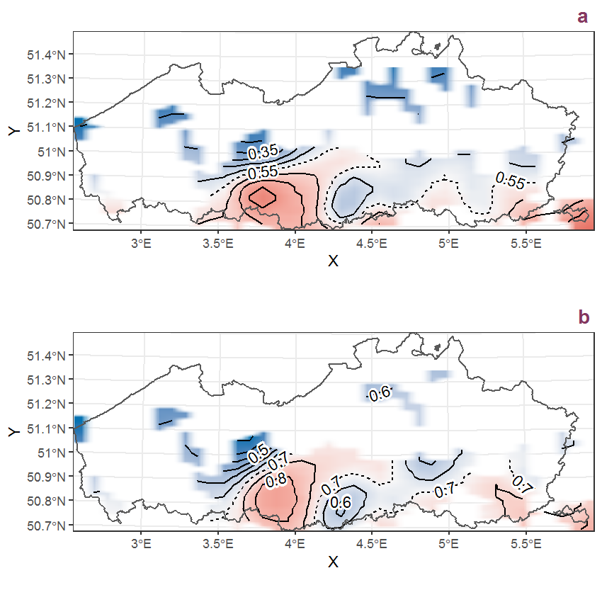
Figure P.27: Visualisation of the spatial smooth effect on the probability of Potentilla sterilis (L.) Garcke presence in 1 km x 1 km squares where the species has been observed at least once. The probabilities (values on the contour lines) are conditional on the final year of observation and a list-length equal to 130. The dashed contour line demarcates zones where the species is expected to be more prevalent (red shades) from zones where the species is less prevalent (blue shades). a: 1950 - 2018, b: 1990 - 2018.
P.10 Primula elatior (L.) Hill
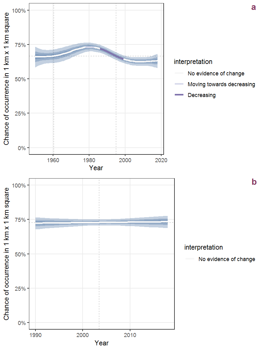
Figure P.28: Effect of year on the probability of Primula elatior (L.) Hill presence in 1 km x 1 km squares where the species has been observed at least once. The fitted line shows the sum of the overall mean (the intercept), a conditional effect of list-length equal to 130 and the year-smoother. The vertical dashed lines indicate the year(s) where the year-smoother is zero. The 95% confidence band is shown in grey (including the variability around the intercept and the smoother). a: 1950 - 2018, b: 1990 - 2018.
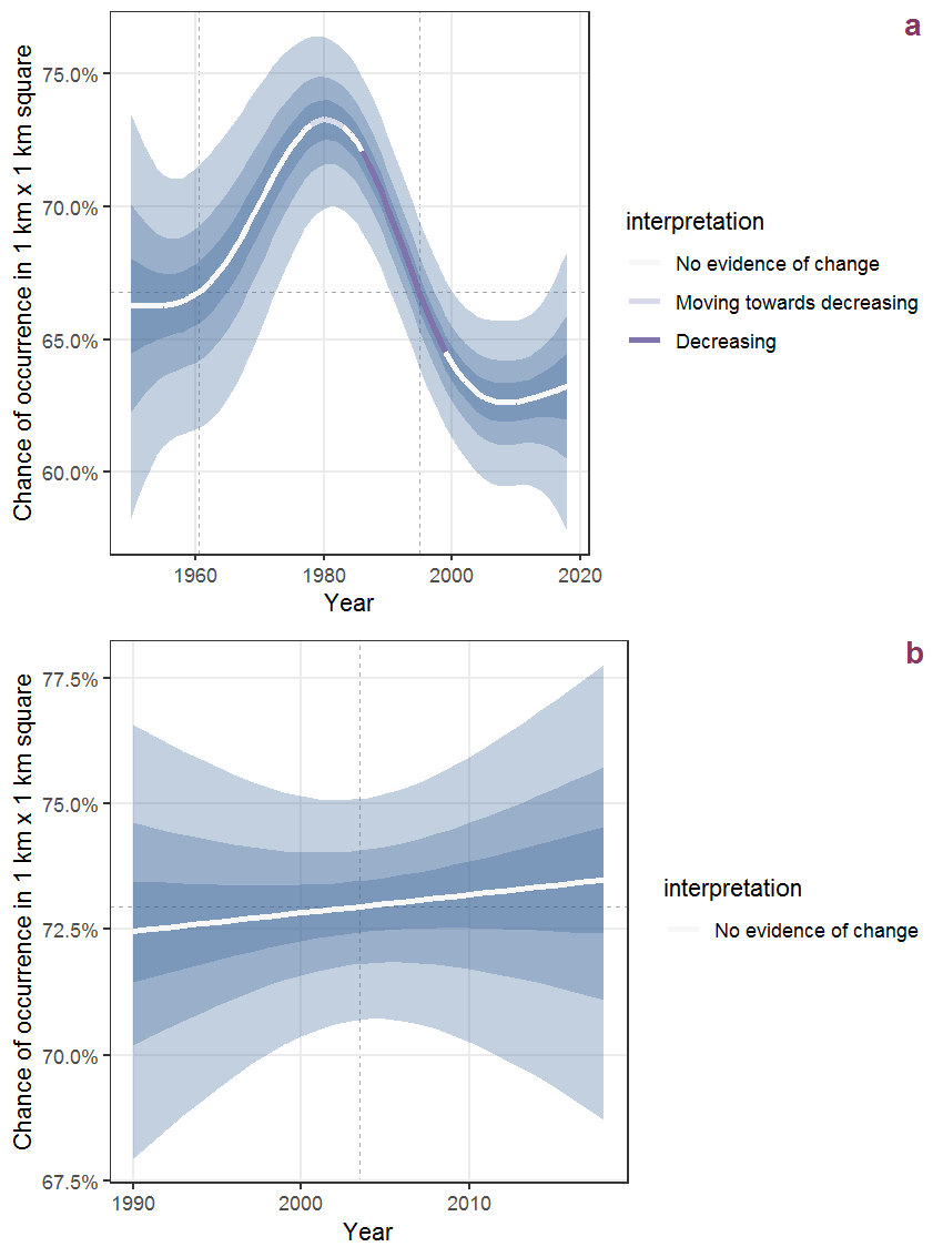
Figure P.29: The same as P.28, but the vertical axis is scaled to the range of the predicted values such that relative changes can be seen more easily. a: 1950 - 2018, b: 1990 - 2018.
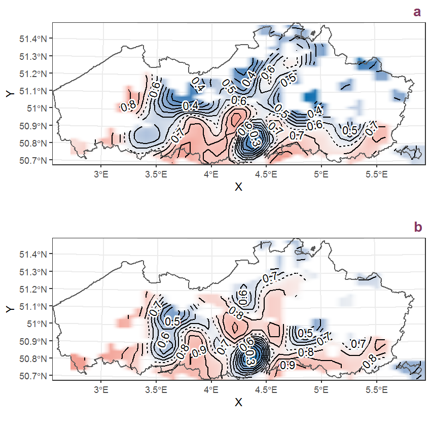
Figure P.30: Visualisation of the spatial smooth effect on the probability of Primula elatior (L.) Hill presence in 1 km x 1 km squares where the species has been observed at least once. The probabilities (values on the contour lines) are conditional on the final year of observation and a list-length equal to 130. The dashed contour line demarcates zones where the species is expected to be more prevalent (red shades) from zones where the species is less prevalent (blue shades). a: 1950 - 2018, b: 1990 - 2018.
P.11 Prunella vulgaris L.
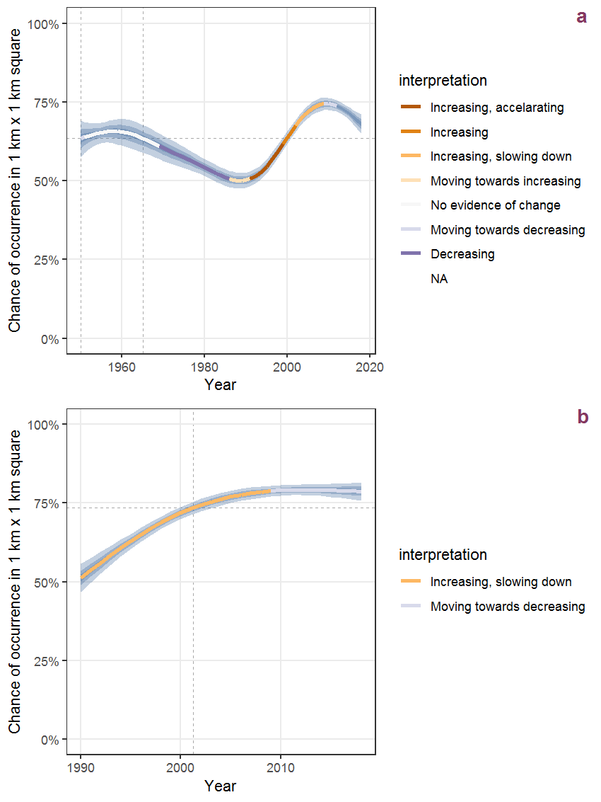
Figure P.31: Effect of year on the probability of Prunella vulgaris L. presence in 1 km x 1 km squares where the species has been observed at least once. The fitted line shows the sum of the overall mean (the intercept), a conditional effect of list-length equal to 130 and the year-smoother. The vertical dashed lines indicate the year(s) where the year-smoother is zero. The 95% confidence band is shown in grey (including the variability around the intercept and the smoother). a: 1950 - 2018, b: 1990 - 2018.
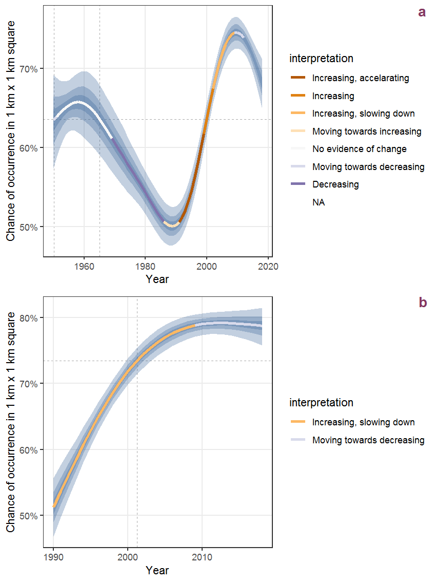
Figure P.32: The same as P.31, but the vertical axis is scaled to the range of the predicted values such that relative changes can be seen more easily. a: 1950 - 2018, b: 1990 - 2018.
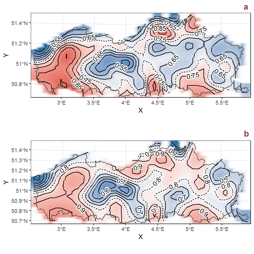
Figure P.33: Visualisation of the spatial smooth effect on the probability of Prunella vulgaris L. presence in 1 km x 1 km squares where the species has been observed at least once. The probabilities (values on the contour lines) are conditional on the final year of observation and a list-length equal to 130. The dashed contour line demarcates zones where the species is expected to be more prevalent (red shades) from zones where the species is less prevalent (blue shades). a: 1950 - 2018, b: 1990 - 2018.
P.12 Prunus avium (L.) L.
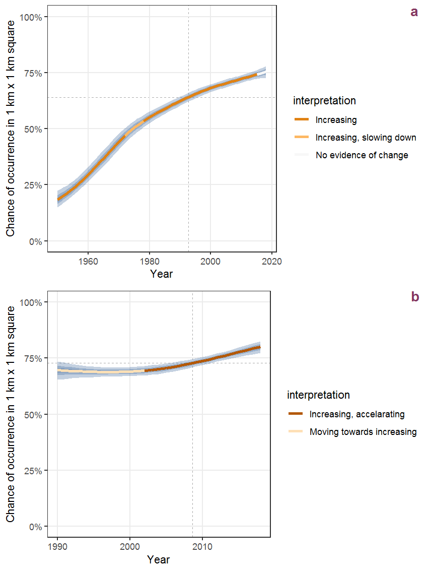
Figure P.34: Effect of year on the probability of Prunus avium (L.) L. presence in 1 km x 1 km squares where the species has been observed at least once. The fitted line shows the sum of the overall mean (the intercept), a conditional effect of list-length equal to 130 and the year-smoother. The vertical dashed lines indicate the year(s) where the year-smoother is zero. The 95% confidence band is shown in grey (including the variability around the intercept and the smoother). a: 1950 - 2018, b: 1990 - 2018.
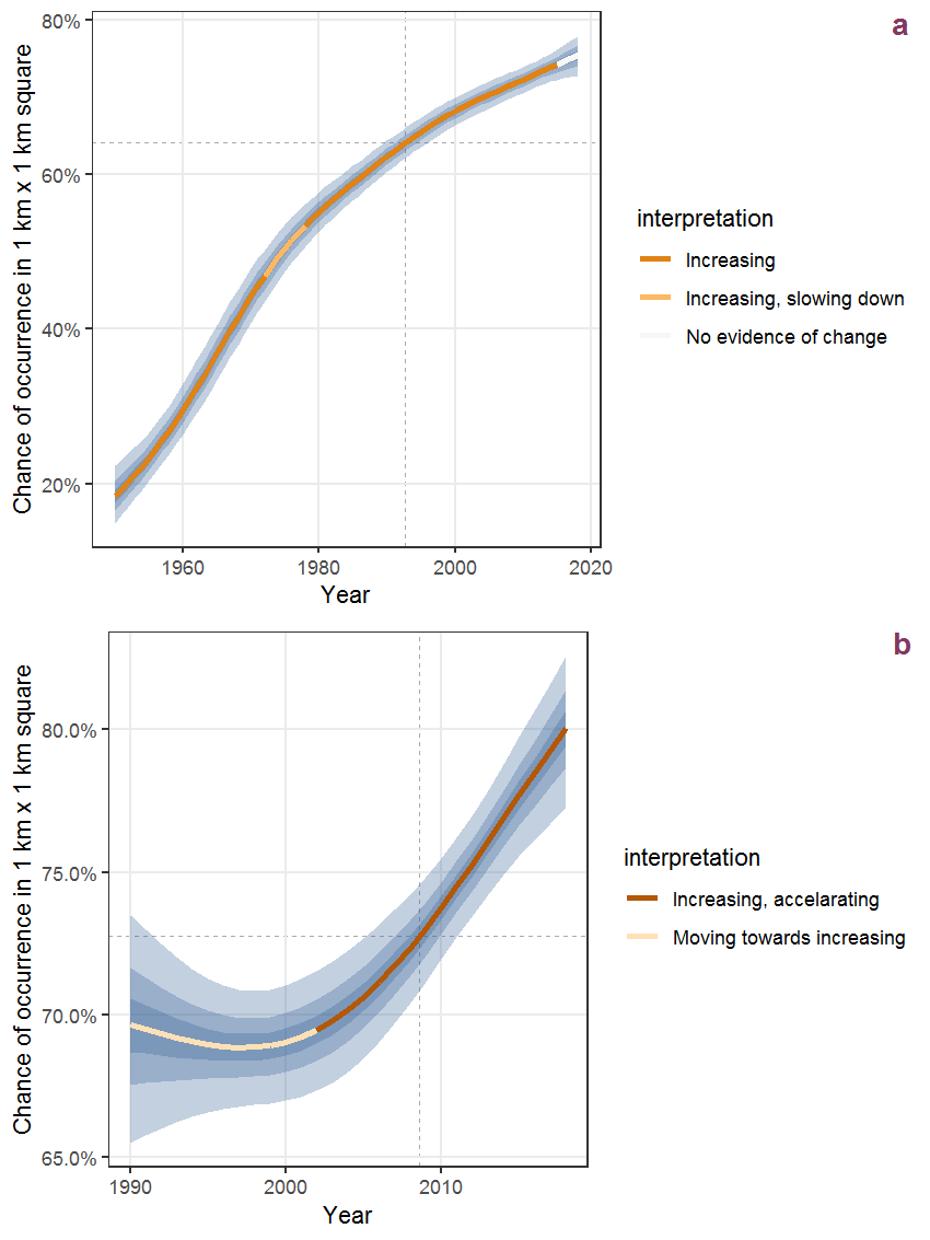
Figure P.35: The same as P.34, but the vertical axis is scaled to the range of the predicted values such that relative changes can be seen more easily. a: 1950 - 2018, b: 1990 - 2018.
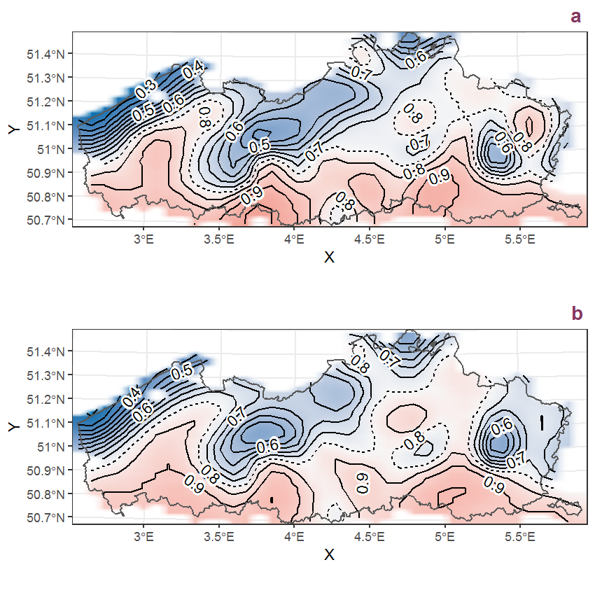
Figure P.36: Visualisation of the spatial smooth effect on the probability of Prunus avium (L.) L. presence in 1 km x 1 km squares where the species has been observed at least once. The probabilities (values on the contour lines) are conditional on the final year of observation and a list-length equal to 130. The dashed contour line demarcates zones where the species is expected to be more prevalent (red shades) from zones where the species is less prevalent (blue shades). a: 1950 - 2018, b: 1990 - 2018.
P.13 Prunus laurocerasus L.
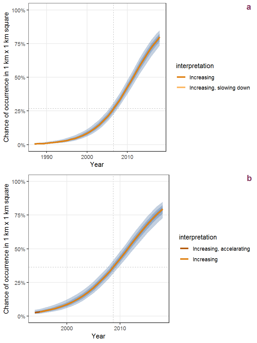
Figure P.37: Effect of year on the probability of Prunus laurocerasus L. presence in 1 km x 1 km squares where the species has been observed at least once. The fitted line shows the sum of the overall mean (the intercept), a conditional effect of list-length equal to 130 and the year-smoother. The vertical dashed lines indicate the year(s) where the year-smoother is zero. The 95% confidence band is shown in grey (including the variability around the intercept and the smoother). a: 1950 - 2018, b: 1990 - 2018.
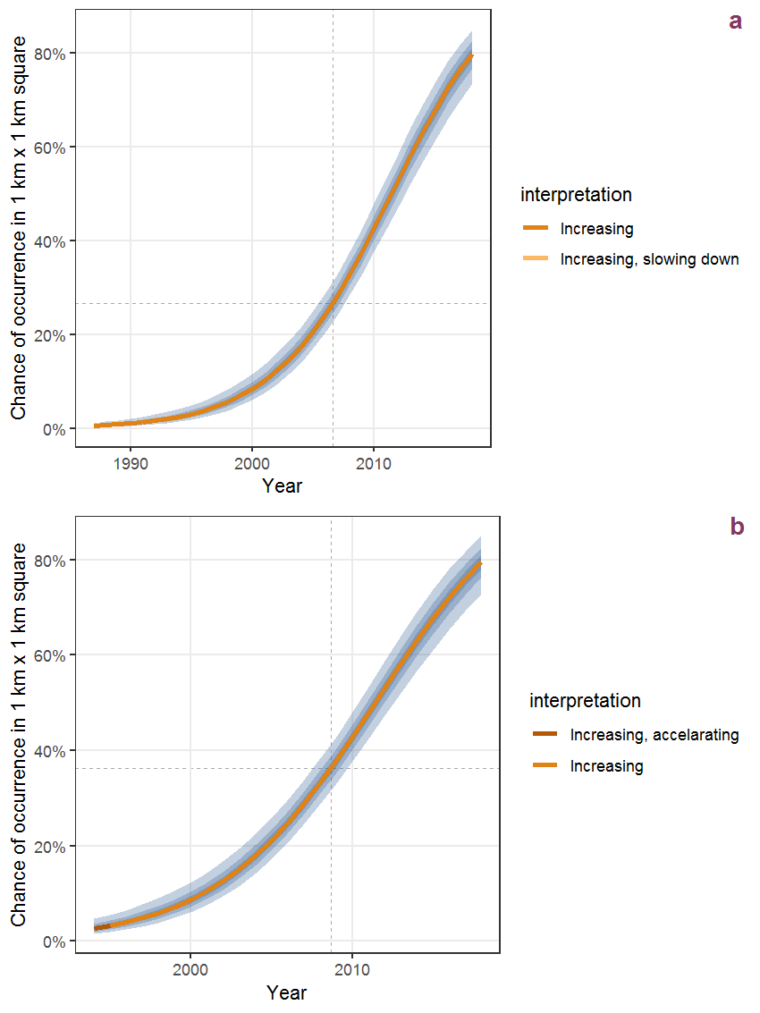
Figure P.38: The same as P.37, but the vertical axis is scaled to the range of the predicted values such that relative changes can be seen more easily. a: 1950 - 2018, b: 1990 - 2018.
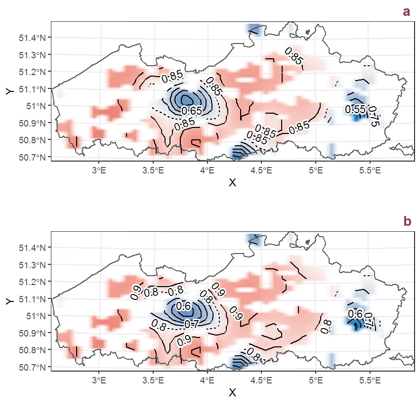
Figure P.39: Visualisation of the spatial smooth effect on the probability of Prunus laurocerasus L. presence in 1 km x 1 km squares where the species has been observed at least once. The probabilities (values on the contour lines) are conditional on the final year of observation and a list-length equal to 130. The dashed contour line demarcates zones where the species is expected to be more prevalent (red shades) from zones where the species is less prevalent (blue shades). a: 1950 - 2018, b: 1990 - 2018.
P.14 Prunus padus L.
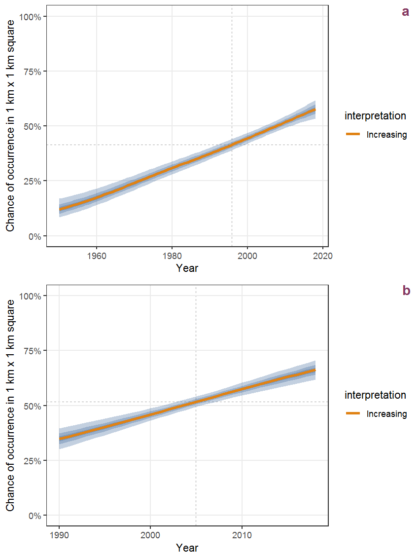
Figure P.40: Effect of year on the probability of Prunus padus L. presence in 1 km x 1 km squares where the species has been observed at least once. The fitted line shows the sum of the overall mean (the intercept), a conditional effect of list-length equal to 130 and the year-smoother. The vertical dashed lines indicate the year(s) where the year-smoother is zero. The 95% confidence band is shown in grey (including the variability around the intercept and the smoother). a: 1950 - 2018, b: 1990 - 2018.
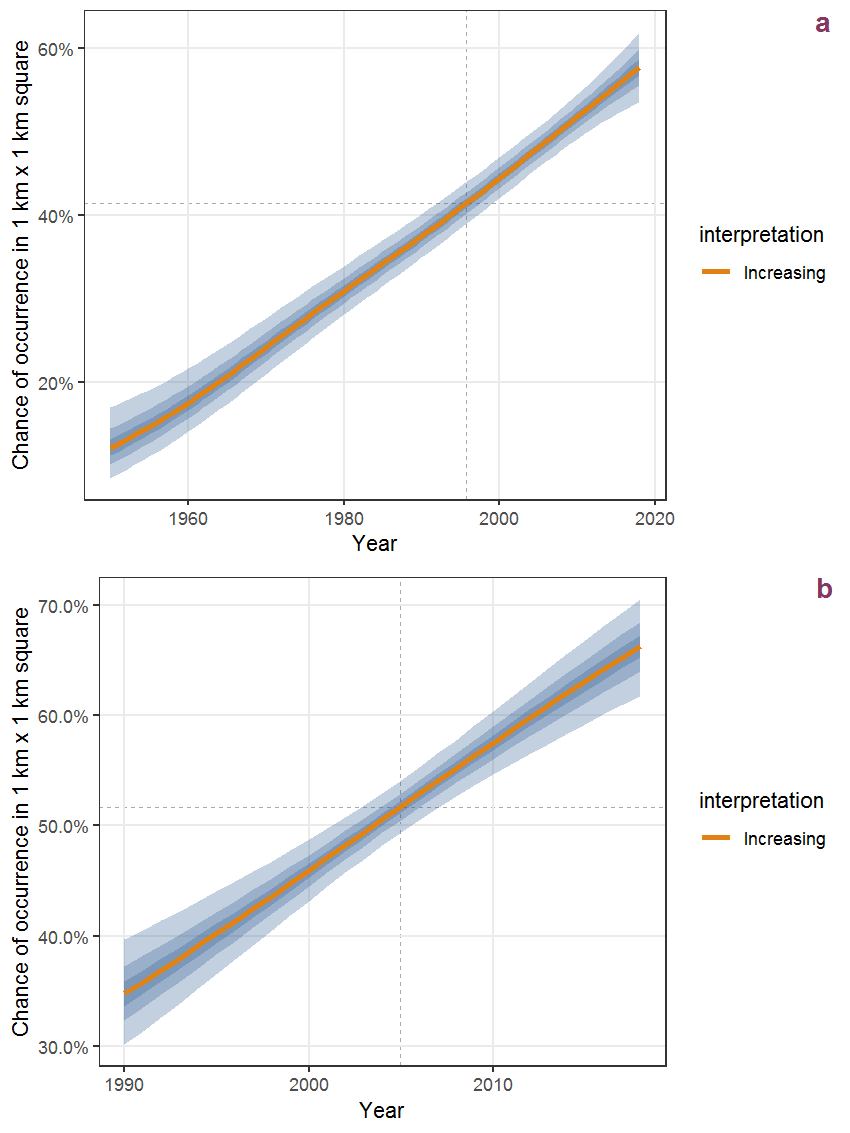
Figure P.41: The same as P.40, but the vertical axis is scaled to the range of the predicted values such that relative changes can be seen more easily. a: 1950 - 2018, b: 1990 - 2018.
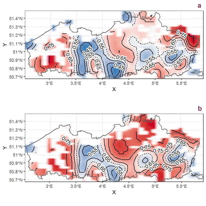
Figure P.42: Visualisation of the spatial smooth effect on the probability of Prunus padus L. presence in 1 km x 1 km squares where the species has been observed at least once. The probabilities (values on the contour lines) are conditional on the final year of observation and a list-length equal to 130. The dashed contour line demarcates zones where the species is expected to be more prevalent (red shades) from zones where the species is less prevalent (blue shades). a: 1950 - 2018, b: 1990 - 2018.
P.15 Prunus serotina Ehrh.
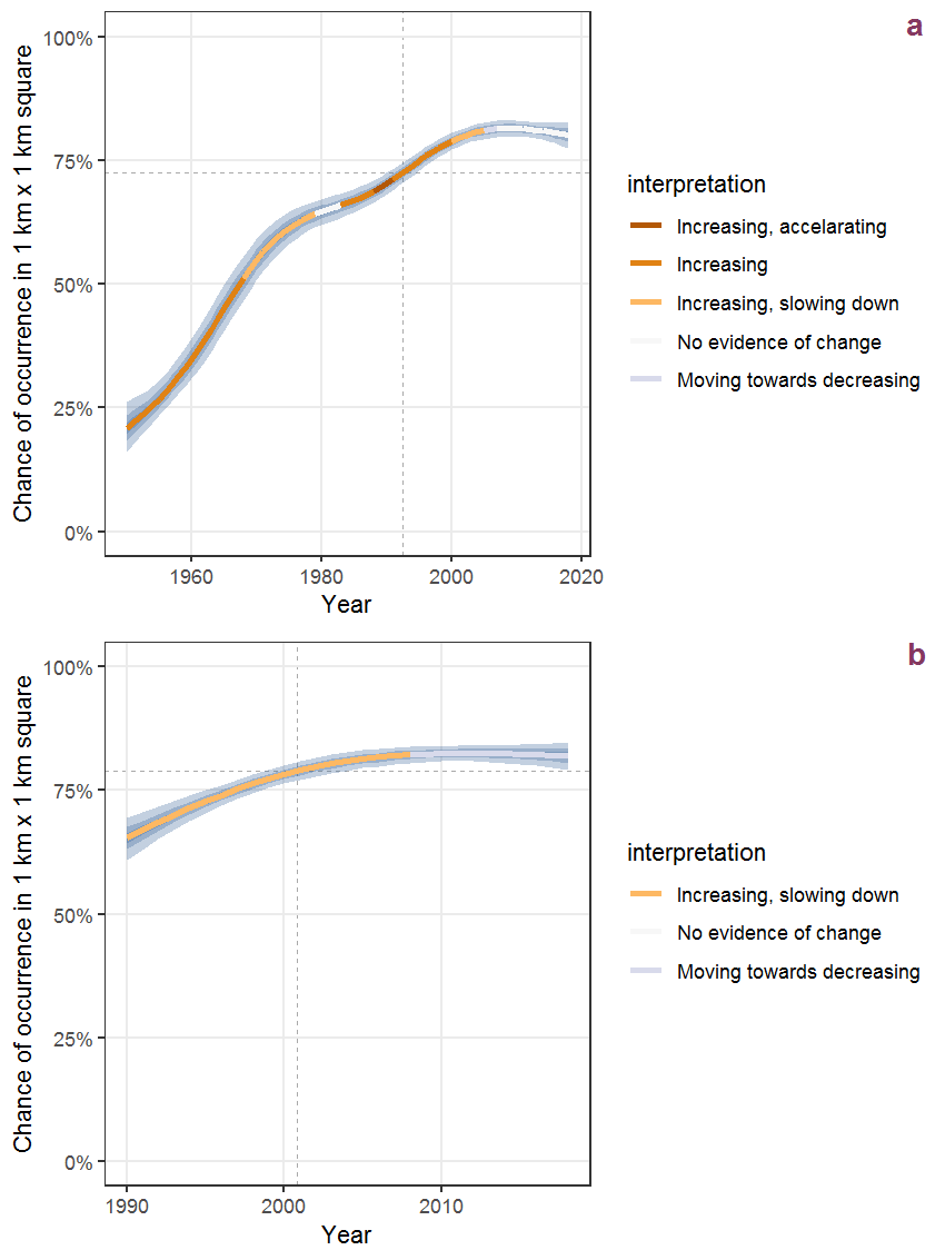
Figure P.43: Effect of year on the probability of Prunus serotina Ehrh. presence in 1 km x 1 km squares where the species has been observed at least once. The fitted line shows the sum of the overall mean (the intercept), a conditional effect of list-length equal to 130 and the year-smoother. The vertical dashed lines indicate the year(s) where the year-smoother is zero. The 95% confidence band is shown in grey (including the variability around the intercept and the smoother). a: 1950 - 2018, b: 1990 - 2018.
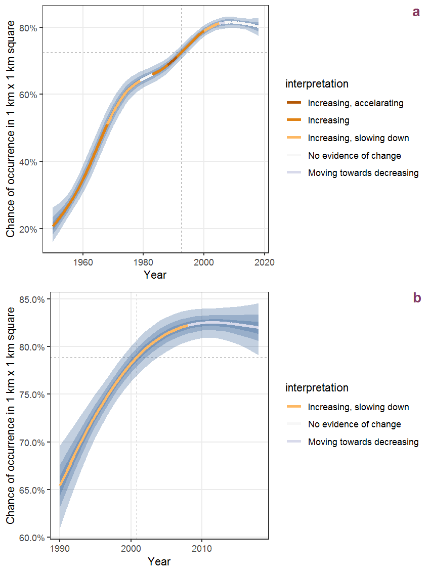
Figure P.44: The same as P.43, but the vertical axis is scaled to the range of the predicted values such that relative changes can be seen more easily. a: 1950 - 2018, b: 1990 - 2018.
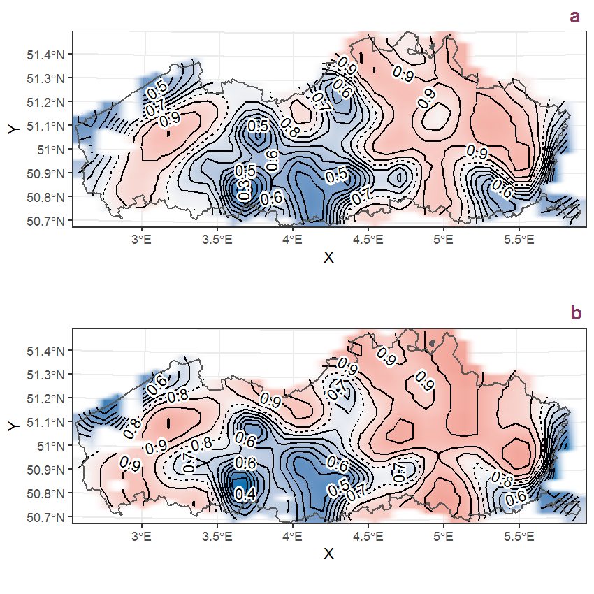
Figure P.45: Visualisation of the spatial smooth effect on the probability of Prunus serotina Ehrh. presence in 1 km x 1 km squares where the species has been observed at least once. The probabilities (values on the contour lines) are conditional on the final year of observation and a list-length equal to 130. The dashed contour line demarcates zones where the species is expected to be more prevalent (red shades) from zones where the species is less prevalent (blue shades). a: 1950 - 2018, b: 1990 - 2018.
P.16 Prunus spinosa L.
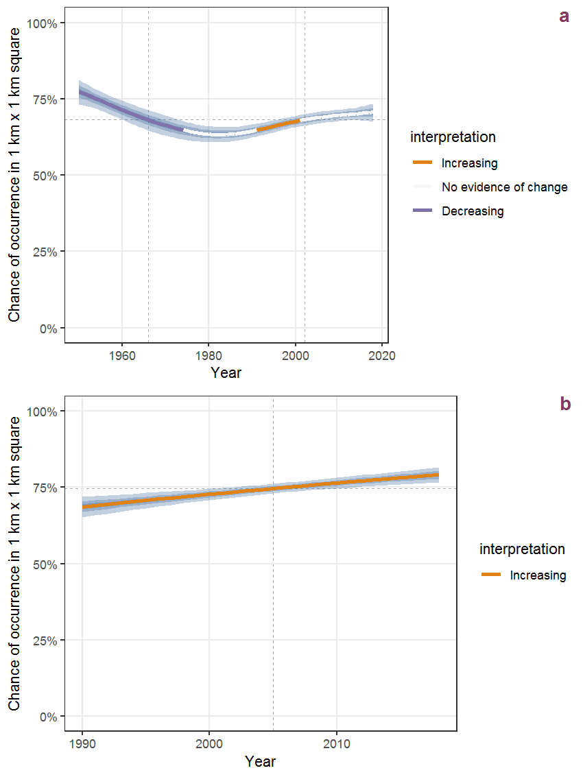
Figure P.46: Effect of year on the probability of Prunus spinosa L. presence in 1 km x 1 km squares where the species has been observed at least once. The fitted line shows the sum of the overall mean (the intercept), a conditional effect of list-length equal to 130 and the year-smoother. The vertical dashed lines indicate the year(s) where the year-smoother is zero. The 95% confidence band is shown in grey (including the variability around the intercept and the smoother). a: 1950 - 2018, b: 1990 - 2018.
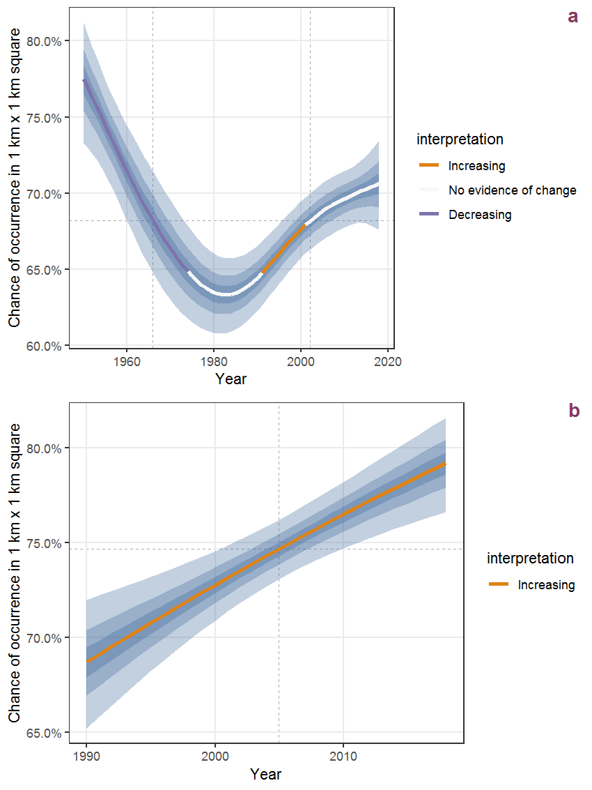
Figure P.47: The same as P.46, but the vertical axis is scaled to the range of the predicted values such that relative changes can be seen more easily. a: 1950 - 2018, b: 1990 - 2018.
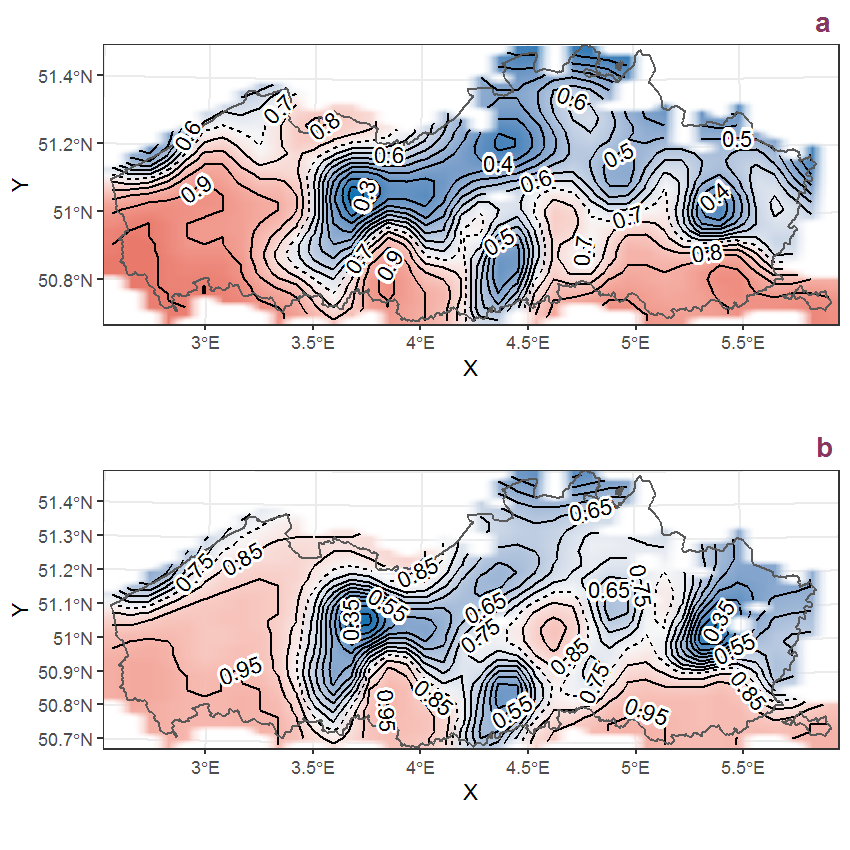
Figure P.48: Visualisation of the spatial smooth effect on the probability of Prunus spinosa L. presence in 1 km x 1 km squares where the species has been observed at least once. The probabilities (values on the contour lines) are conditional on the final year of observation and a list-length equal to 130. The dashed contour line demarcates zones where the species is expected to be more prevalent (red shades) from zones where the species is less prevalent (blue shades). a: 1950 - 2018, b: 1990 - 2018.
P.17 Pseudofumaria lutea (L.) Borkh.
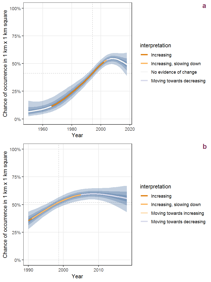
Figure P.49: Effect of year on the probability of Pseudofumaria lutea (L.) Borkh. presence in 1 km x 1 km squares where the species has been observed at least once. The fitted line shows the sum of the overall mean (the intercept), a conditional effect of list-length equal to 130 and the year-smoother. The vertical dashed lines indicate the year(s) where the year-smoother is zero. The 95% confidence band is shown in grey (including the variability around the intercept and the smoother). a: 1950 - 2018, b: 1990 - 2018.
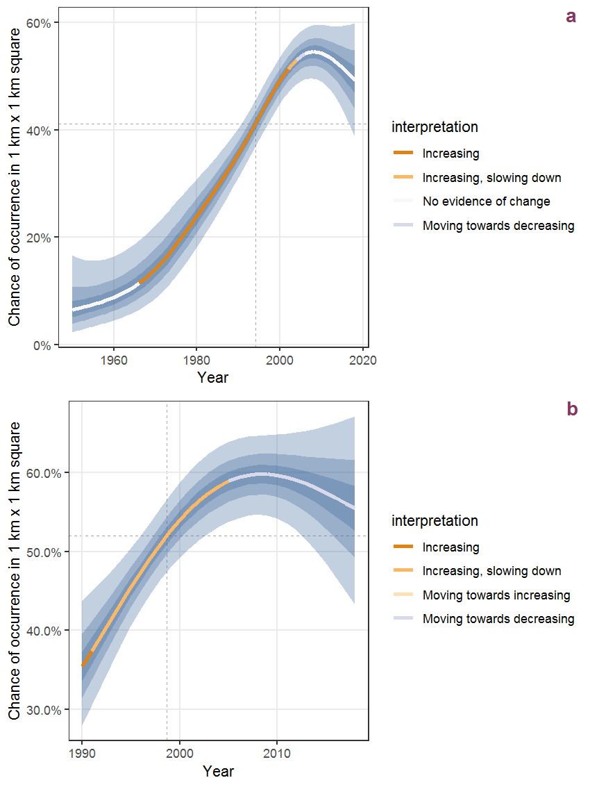
Figure P.50: The same as P.49, but the vertical axis is scaled to the range of the predicted values such that relative changes can be seen more easily. a: 1950 - 2018, b: 1990 - 2018.
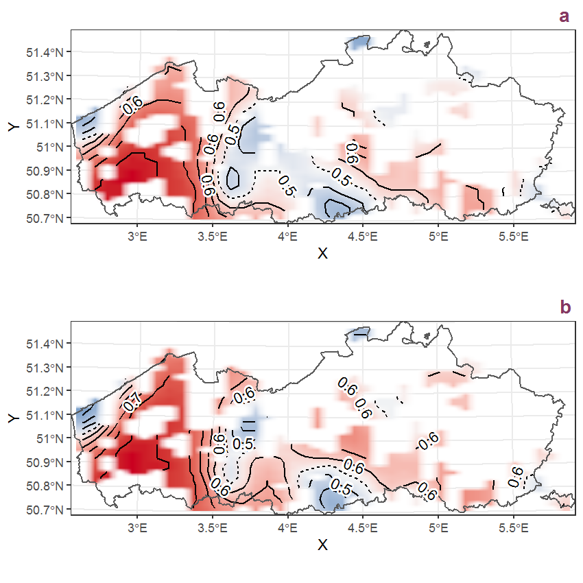
Figure P.51: Visualisation of the spatial smooth effect on the probability of Pseudofumaria lutea (L.) Borkh. presence in 1 km x 1 km squares where the species has been observed at least once. The probabilities (values on the contour lines) are conditional on the final year of observation and a list-length equal to 130. The dashed contour line demarcates zones where the species is expected to be more prevalent (red shades) from zones where the species is less prevalent (blue shades). a: 1950 - 2018, b: 1990 - 2018.
P.18 Pteridium aquilinum (L.) Kuhn
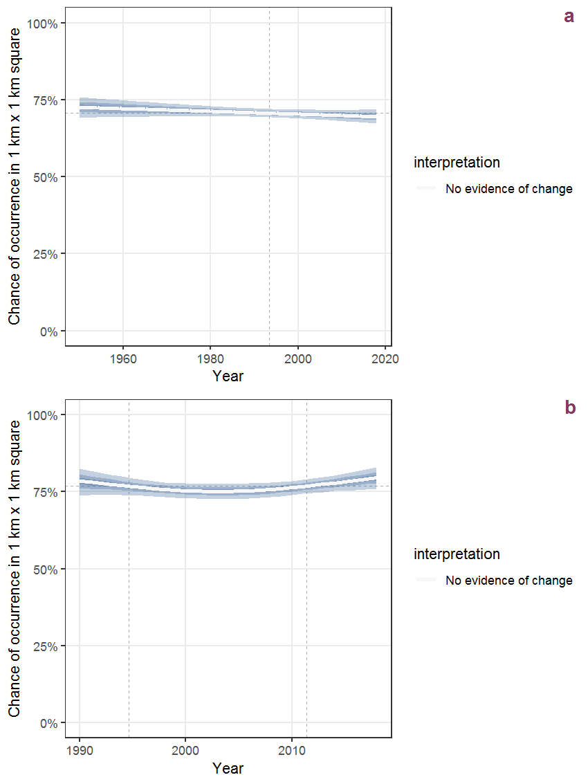
Figure P.52: Effect of year on the probability of Pteridium aquilinum (L.) Kuhn presence in 1 km x 1 km squares where the species has been observed at least once. The fitted line shows the sum of the overall mean (the intercept), a conditional effect of list-length equal to 130 and the year-smoother. The vertical dashed lines indicate the year(s) where the year-smoother is zero. The 95% confidence band is shown in grey (including the variability around the intercept and the smoother). a: 1950 - 2018, b: 1990 - 2018.
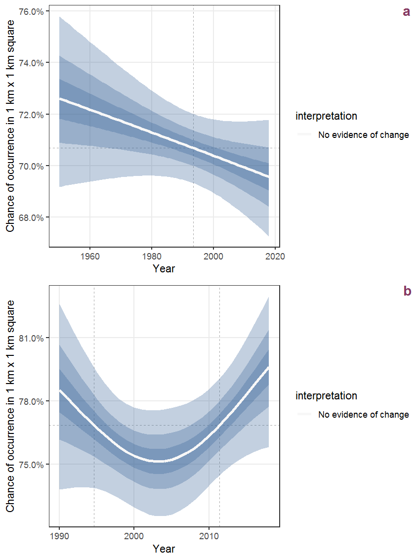
Figure P.53: The same as P.52, but the vertical axis is scaled to the range of the predicted values such that relative changes can be seen more easily. a: 1950 - 2018, b: 1990 - 2018.
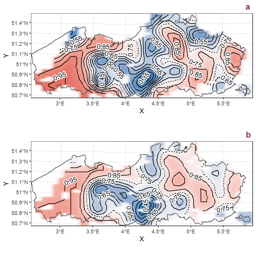
Figure P.54: Visualisation of the spatial smooth effect on the probability of Pteridium aquilinum (L.) Kuhn presence in 1 km x 1 km squares where the species has been observed at least once. The probabilities (values on the contour lines) are conditional on the final year of observation and a list-length equal to 130. The dashed contour line demarcates zones where the species is expected to be more prevalent (red shades) from zones where the species is less prevalent (blue shades). a: 1950 - 2018, b: 1990 - 2018.
P.19 Pulicaria dysenterica (L.) Bernh.
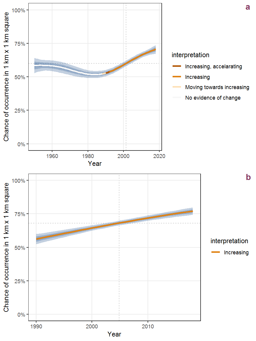
Figure P.55: Effect of year on the probability of Pulicaria dysenterica (L.) Bernh. presence in 1 km x 1 km squares where the species has been observed at least once. The fitted line shows the sum of the overall mean (the intercept), a conditional effect of list-length equal to 130 and the year-smoother. The vertical dashed lines indicate the year(s) where the year-smoother is zero. The 95% confidence band is shown in grey (including the variability around the intercept and the smoother). a: 1950 - 2018, b: 1990 - 2018.
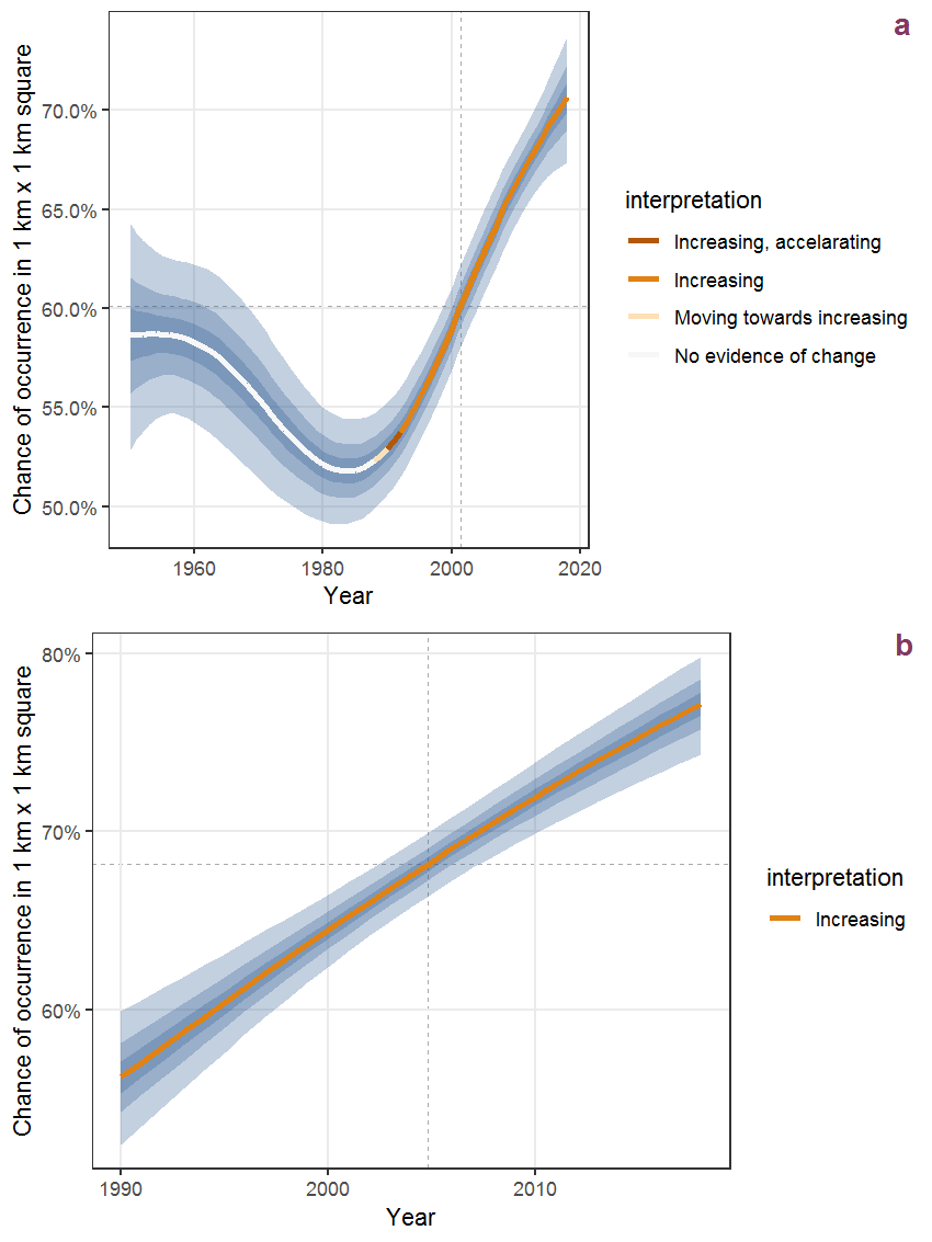
Figure P.56: The same as P.55, but the vertical axis is scaled to the range of the predicted values such that relative changes can be seen more easily. a: 1950 - 2018, b: 1990 - 2018.
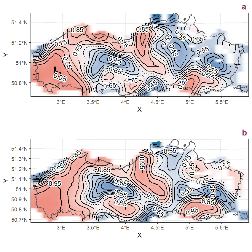
Figure P.57: Visualisation of the spatial smooth effect on the probability of Pulicaria dysenterica (L.) Bernh. presence in 1 km x 1 km squares where the species has been observed at least once. The probabilities (values on the contour lines) are conditional on the final year of observation and a list-length equal to 130. The dashed contour line demarcates zones where the species is expected to be more prevalent (red shades) from zones where the species is less prevalent (blue shades). a: 1950 - 2018, b: 1990 - 2018.
P.20 Quercus petraea Lieblein
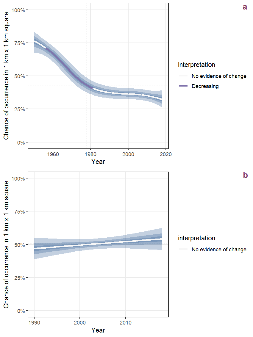
Figure P.58: Effect of year on the probability of Quercus petraea Lieblein presence in 1 km x 1 km squares where the species has been observed at least once. The fitted line shows the sum of the overall mean (the intercept), a conditional effect of list-length equal to 130 and the year-smoother. The vertical dashed lines indicate the year(s) where the year-smoother is zero. The 95% confidence band is shown in grey (including the variability around the intercept and the smoother). a: 1950 - 2018, b: 1990 - 2018.
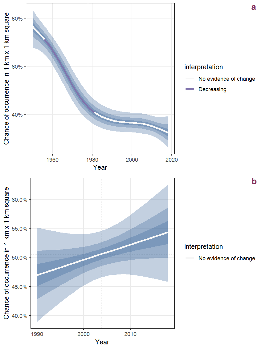
Figure P.59: The same as P.58, but the vertical axis is scaled to the range of the predicted values such that relative changes can be seen more easily. a: 1950 - 2018, b: 1990 - 2018.

Figure P.60: Visualisation of the spatial smooth effect on the probability of Quercus petraea Lieblein presence in 1 km x 1 km squares where the species has been observed at least once. The probabilities (values on the contour lines) are conditional on the final year of observation and a list-length equal to 130. The dashed contour line demarcates zones where the species is expected to be more prevalent (red shades) from zones where the species is less prevalent (blue shades). a: 1950 - 2018, b: 1990 - 2018.
P.21 Quercus robur L.
Figure P.61: Effect of year on the probability of Quercus robur L. presence in 1 km x 1 km squares where the species has been observed at least once. The fitted line shows the sum of the overall mean (the intercept), a conditional effect of list-length equal to 130 and the year-smoother. The vertical dashed lines indicate the year(s) where the year-smoother is zero. The 95% confidence band is shown in grey (including the variability around the intercept and the smoother). a: 1950 - 2018, b: 1990 - 2018.
Figure P.62: The same as P.61, but the vertical axis is scaled to the range of the predicted values such that relative changes can be seen more easily. a: 1950 - 2018, b: 1990 - 2018.
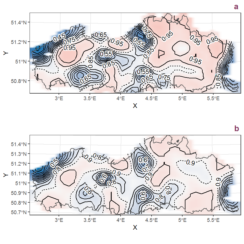
Figure P.63: Visualisation of the spatial smooth effect on the probability of Quercus robur L. presence in 1 km x 1 km squares where the species has been observed at least once. The probabilities (values on the contour lines) are conditional on the final year of observation and a list-length equal to 130. The dashed contour line demarcates zones where the species is expected to be more prevalent (red shades) from zones where the species is less prevalent (blue shades). a: 1950 - 2018, b: 1990 - 2018.
P.22 Quercus rubra L.
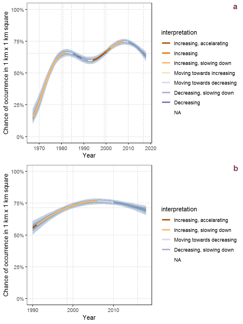
Figure P.64: Effect of year on the probability of Quercus rubra L. presence in 1 km x 1 km squares where the species has been observed at least once. The fitted line shows the sum of the overall mean (the intercept), a conditional effect of list-length equal to 130 and the year-smoother. The vertical dashed lines indicate the year(s) where the year-smoother is zero. The 95% confidence band is shown in grey (including the variability around the intercept and the smoother). a: 1950 - 2018, b: 1990 - 2018.
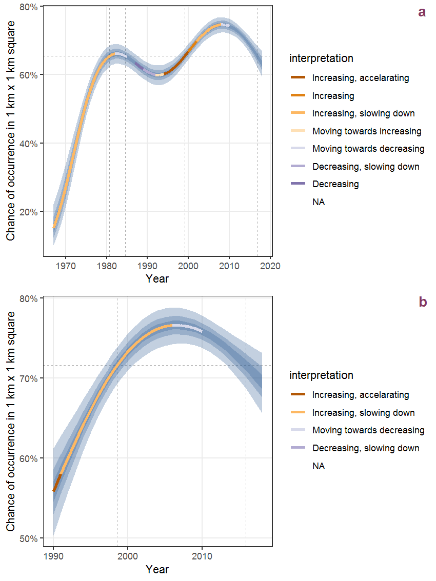
Figure P.65: The same as P.64, but the vertical axis is scaled to the range of the predicted values such that relative changes can be seen more easily. a: 1950 - 2018, b: 1990 - 2018.
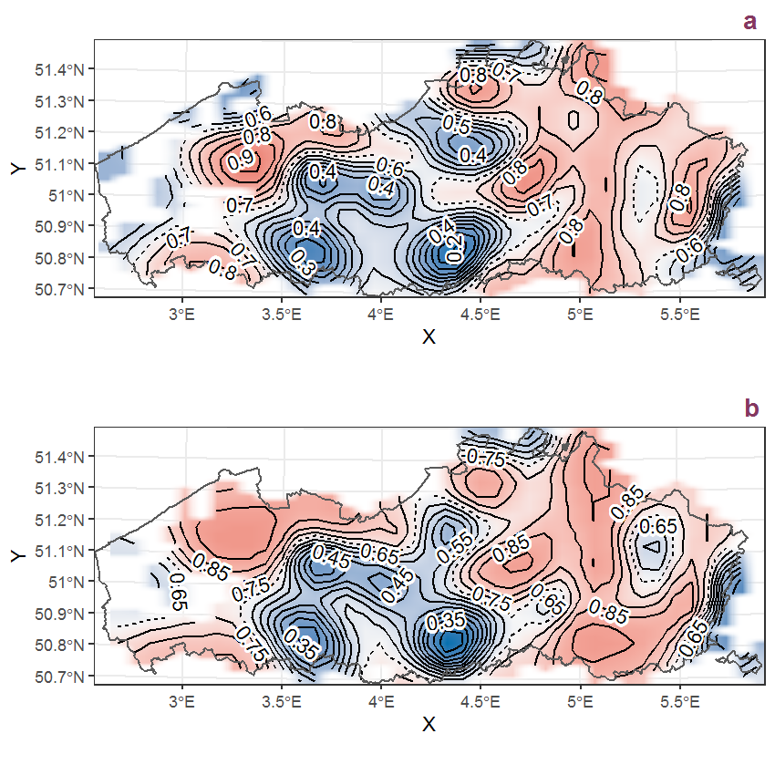
Figure P.66: Visualisation of the spatial smooth effect on the probability of Quercus rubra L. presence in 1 km x 1 km squares where the species has been observed at least once. The probabilities (values on the contour lines) are conditional on the final year of observation and a list-length equal to 130. The dashed contour line demarcates zones where the species is expected to be more prevalent (red shades) from zones where the species is less prevalent (blue shades). a: 1950 - 2018, b: 1990 - 2018.
P.23 Ranunculus acris L.
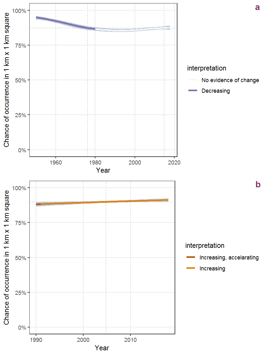
Figure P.67: Effect of year on the probability of Ranunculus acris L. presence in 1 km x 1 km squares where the species has been observed at least once. The fitted line shows the sum of the overall mean (the intercept), a conditional effect of list-length equal to 130 and the year-smoother. The vertical dashed lines indicate the year(s) where the year-smoother is zero. The 95% confidence band is shown in grey (including the variability around the intercept and the smoother). a: 1950 - 2018, b: 1990 - 2018.
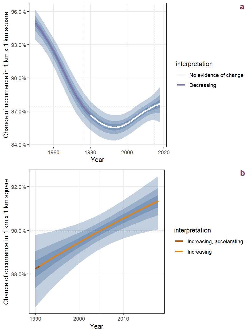
Figure P.68: The same as P.67, but the vertical axis is scaled to the range of the predicted values such that relative changes can be seen more easily. a: 1950 - 2018, b: 1990 - 2018.
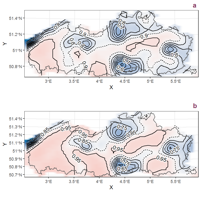
Figure P.69: Visualisation of the spatial smooth effect on the probability of Ranunculus acris L. presence in 1 km x 1 km squares where the species has been observed at least once. The probabilities (values on the contour lines) are conditional on the final year of observation and a list-length equal to 130. The dashed contour line demarcates zones where the species is expected to be more prevalent (red shades) from zones where the species is less prevalent (blue shades). a: 1950 - 2018, b: 1990 - 2018.
P.24 Ranunculus aquatilis L.
Figure P.70: Effect of year on the probability of Ranunculus aquatilis L. presence in 1 km x 1 km squares where the species has been observed at least once. The fitted line shows the sum of the overall mean (the intercept), a conditional effect of list-length equal to 130 and the year-smoother. The vertical dashed lines indicate the year(s) where the year-smoother is zero. The 95% confidence band is shown in grey (including the variability around the intercept and the smoother). a: 1950 - 2018, b: 1990 - 2018.
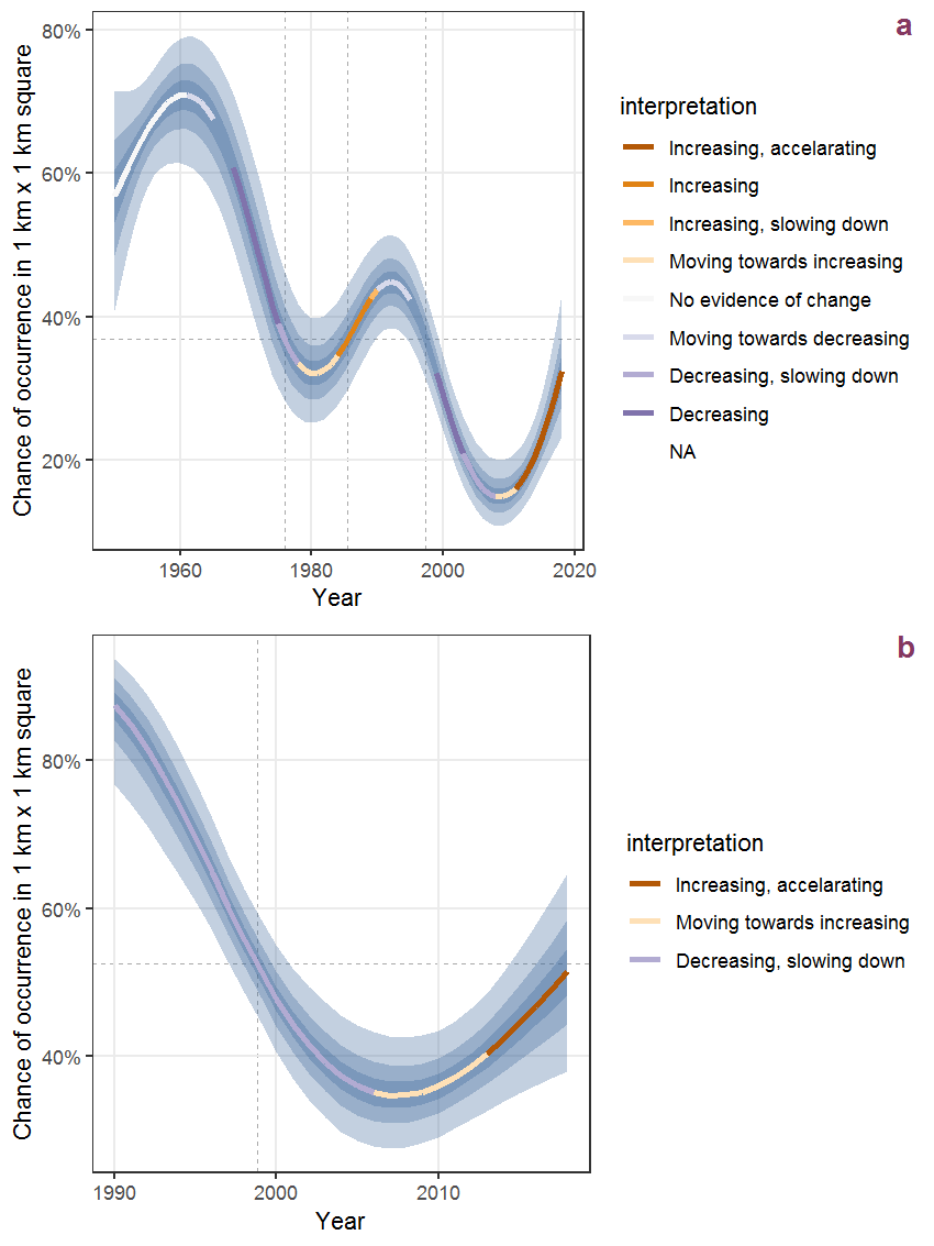
Figure P.71: The same as P.70, but the vertical axis is scaled to the range of the predicted values such that relative changes can be seen more easily. a: 1950 - 2018, b: 1990 - 2018.
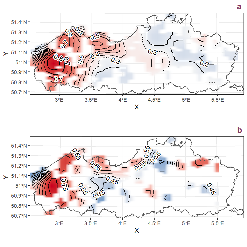
Figure P.72: Visualisation of the spatial smooth effect on the probability of Ranunculus aquatilis L. presence in 1 km x 1 km squares where the species has been observed at least once. The probabilities (values on the contour lines) are conditional on the final year of observation and a list-length equal to 130. The dashed contour line demarcates zones where the species is expected to be more prevalent (red shades) from zones where the species is less prevalent (blue shades). a: 1950 - 2018, b: 1990 - 2018.
P.25 Ranunculus auricomus L.
Figure P.73: Effect of year on the probability of Ranunculus auricomus L. presence in 1 km x 1 km squares where the species has been observed at least once. The fitted line shows the sum of the overall mean (the intercept), a conditional effect of list-length equal to 130 and the year-smoother. The vertical dashed lines indicate the year(s) where the year-smoother is zero. The 95% confidence band is shown in grey (including the variability around the intercept and the smoother). a: 1950 - 2018, b: 1990 - 2018.
Figure P.74: The same as P.73, but the vertical axis is scaled to the range of the predicted values such that relative changes can be seen more easily. a: 1950 - 2018, b: 1990 - 2018.
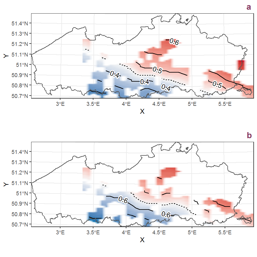
Figure P.75: Visualisation of the spatial smooth effect on the probability of Ranunculus auricomus L. presence in 1 km x 1 km squares where the species has been observed at least once. The probabilities (values on the contour lines) are conditional on the final year of observation and a list-length equal to 130. The dashed contour line demarcates zones where the species is expected to be more prevalent (red shades) from zones where the species is less prevalent (blue shades). a: 1950 - 2018, b: 1990 - 2018.
P.26 Ranunculus bulbosus L.
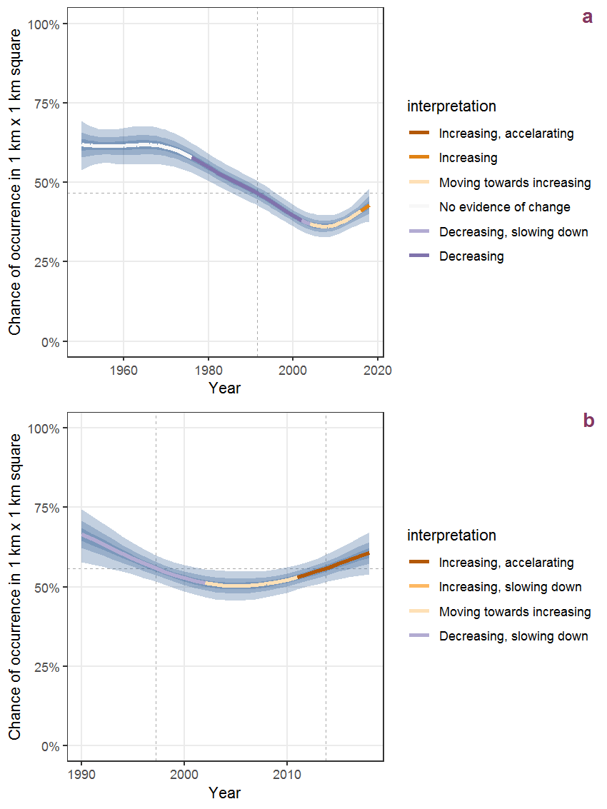
Figure P.76: Effect of year on the probability of Ranunculus bulbosus L. presence in 1 km x 1 km squares where the species has been observed at least once. The fitted line shows the sum of the overall mean (the intercept), a conditional effect of list-length equal to 130 and the year-smoother. The vertical dashed lines indicate the year(s) where the year-smoother is zero. The 95% confidence band is shown in grey (including the variability around the intercept and the smoother). a: 1950 - 2018, b: 1990 - 2018.
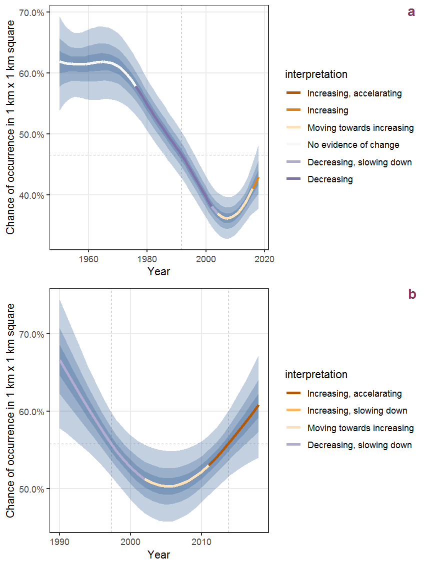
Figure P.77: The same as P.76, but the vertical axis is scaled to the range of the predicted values such that relative changes can be seen more easily. a: 1950 - 2018, b: 1990 - 2018.
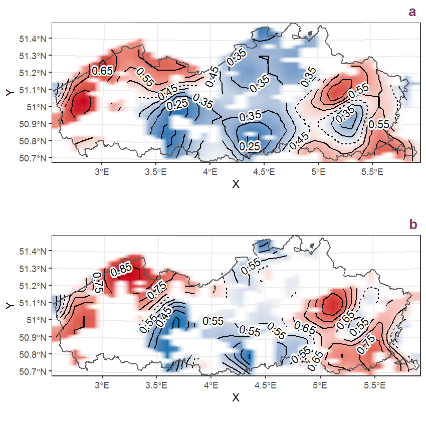
Figure P.78: Visualisation of the spatial smooth effect on the probability of Ranunculus bulbosus L. presence in 1 km x 1 km squares where the species has been observed at least once. The probabilities (values on the contour lines) are conditional on the final year of observation and a list-length equal to 130. The dashed contour line demarcates zones where the species is expected to be more prevalent (red shades) from zones where the species is less prevalent (blue shades). a: 1950 - 2018, b: 1990 - 2018.
P.27 Ranunculus ficaria L.
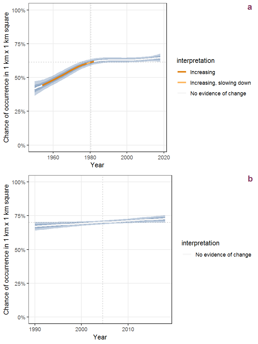
Figure P.79: Effect of year on the probability of Ranunculus ficaria L. presence in 1 km x 1 km squares where the species has been observed at least once. The fitted line shows the sum of the overall mean (the intercept), a conditional effect of list-length equal to 130 and the year-smoother. The vertical dashed lines indicate the year(s) where the year-smoother is zero. The 95% confidence band is shown in grey (including the variability around the intercept and the smoother). a: 1950 - 2018, b: 1990 - 2018.
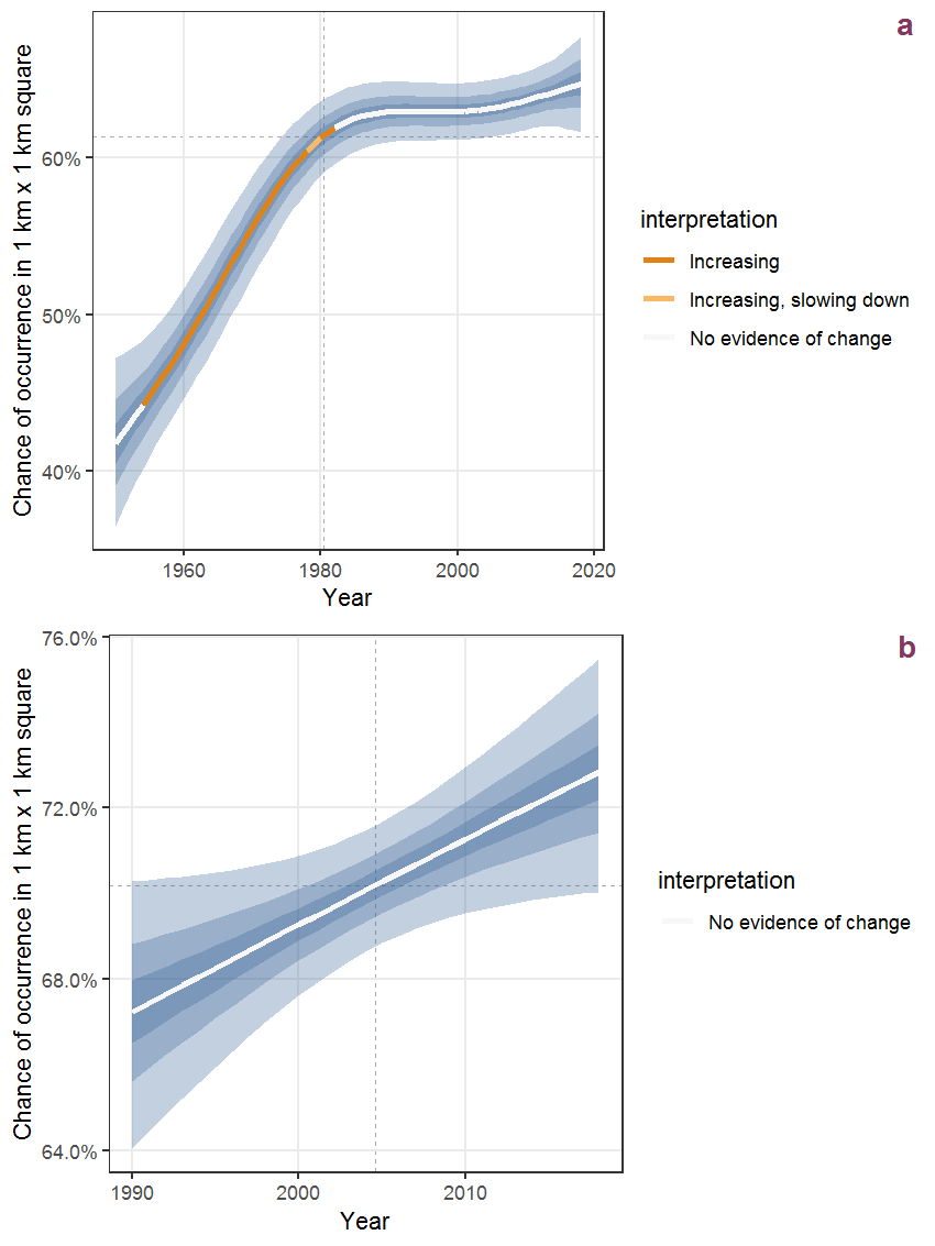
Figure P.80: The same as P.79, but the vertical axis is scaled to the range of the predicted values such that relative changes can be seen more easily. a: 1950 - 2018, b: 1990 - 2018.
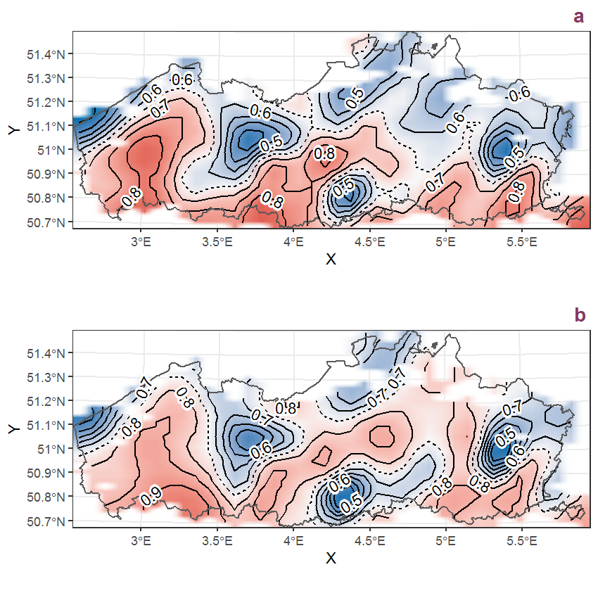
Figure P.81: Visualisation of the spatial smooth effect on the probability of Ranunculus ficaria L. presence in 1 km x 1 km squares where the species has been observed at least once. The probabilities (values on the contour lines) are conditional on the final year of observation and a list-length equal to 130. The dashed contour line demarcates zones where the species is expected to be more prevalent (red shades) from zones where the species is less prevalent (blue shades). a: 1950 - 2018, b: 1990 - 2018.
P.28 Ranunculus flammula L.
Figure P.82: Effect of year on the probability of Ranunculus flammula L. presence in 1 km x 1 km squares where the species has been observed at least once. The fitted line shows the sum of the overall mean (the intercept), a conditional effect of list-length equal to 130 and the year-smoother. The vertical dashed lines indicate the year(s) where the year-smoother is zero. The 95% confidence band is shown in grey (including the variability around the intercept and the smoother). a: 1950 - 2018, b: 1990 - 2018.
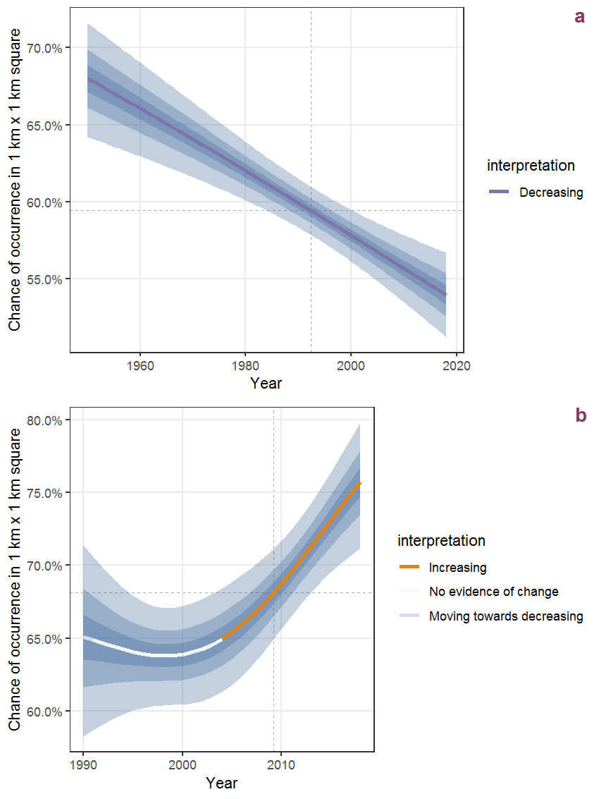
Figure P.83: The same as P.82, but the vertical axis is scaled to the range of the predicted values such that relative changes can be seen more easily. a: 1950 - 2018, b: 1990 - 2018.
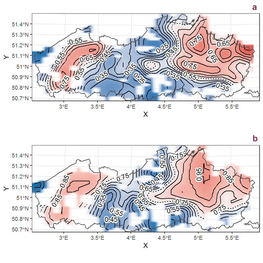
Figure P.84: Visualisation of the spatial smooth effect on the probability of Ranunculus flammula L. presence in 1 km x 1 km squares where the species has been observed at least once. The probabilities (values on the contour lines) are conditional on the final year of observation and a list-length equal to 130. The dashed contour line demarcates zones where the species is expected to be more prevalent (red shades) from zones where the species is less prevalent (blue shades). a: 1950 - 2018, b: 1990 - 2018.
P.29 Ranunculus repens L.
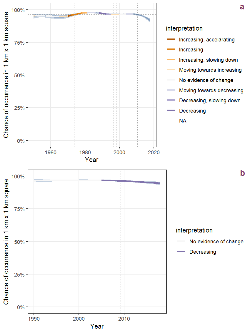
Figure P.85: Effect of year on the probability of Ranunculus repens L. presence in 1 km x 1 km squares where the species has been observed at least once. The fitted line shows the sum of the overall mean (the intercept), a conditional effect of list-length equal to 130 and the year-smoother. The vertical dashed lines indicate the year(s) where the year-smoother is zero. The 95% confidence band is shown in grey (including the variability around the intercept and the smoother). a: 1950 - 2018, b: 1990 - 2018.
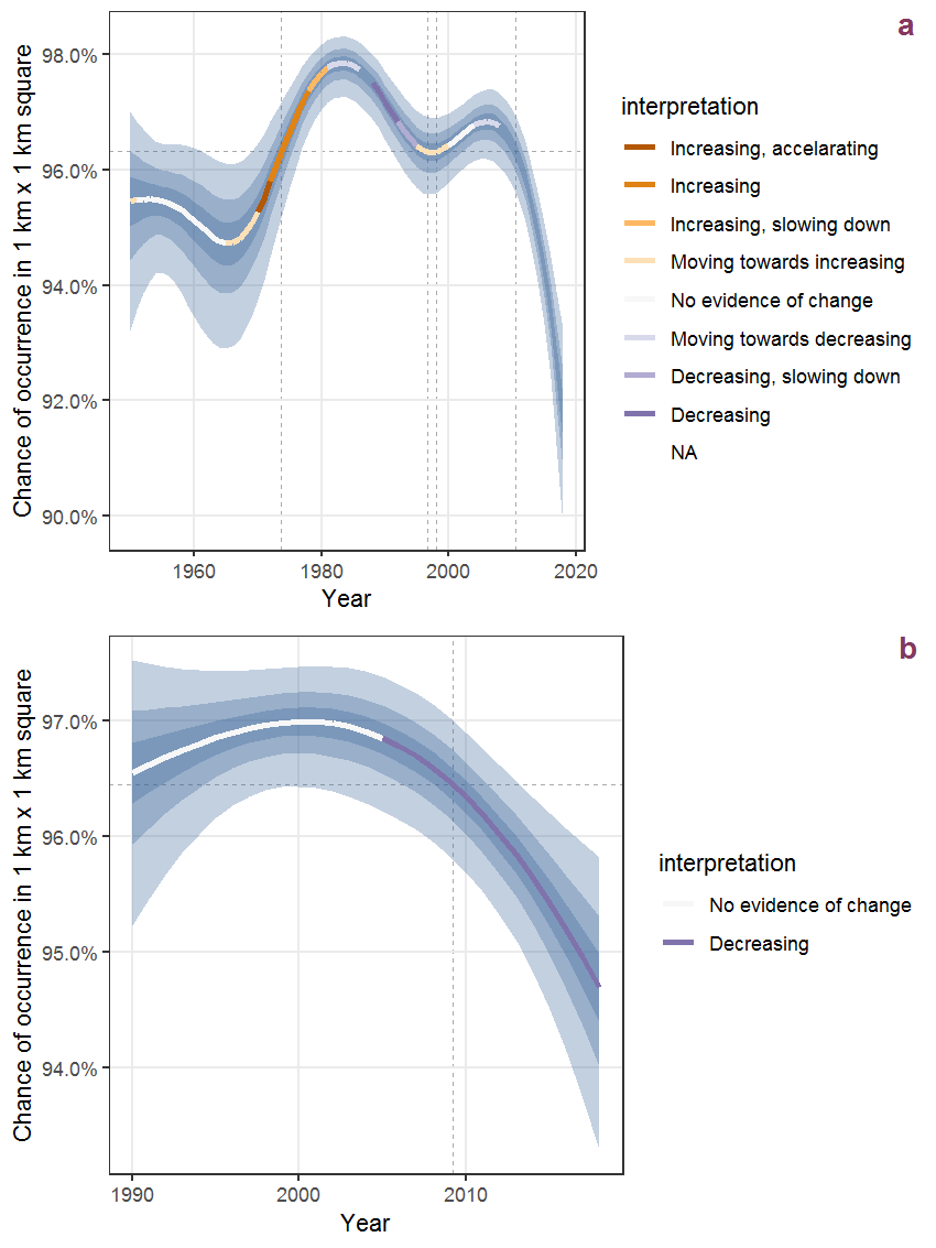
Figure P.86: The same as P.85, but the vertical axis is scaled to the range of the predicted values such that relative changes can be seen more easily. a: 1950 - 2018, b: 1990 - 2018.
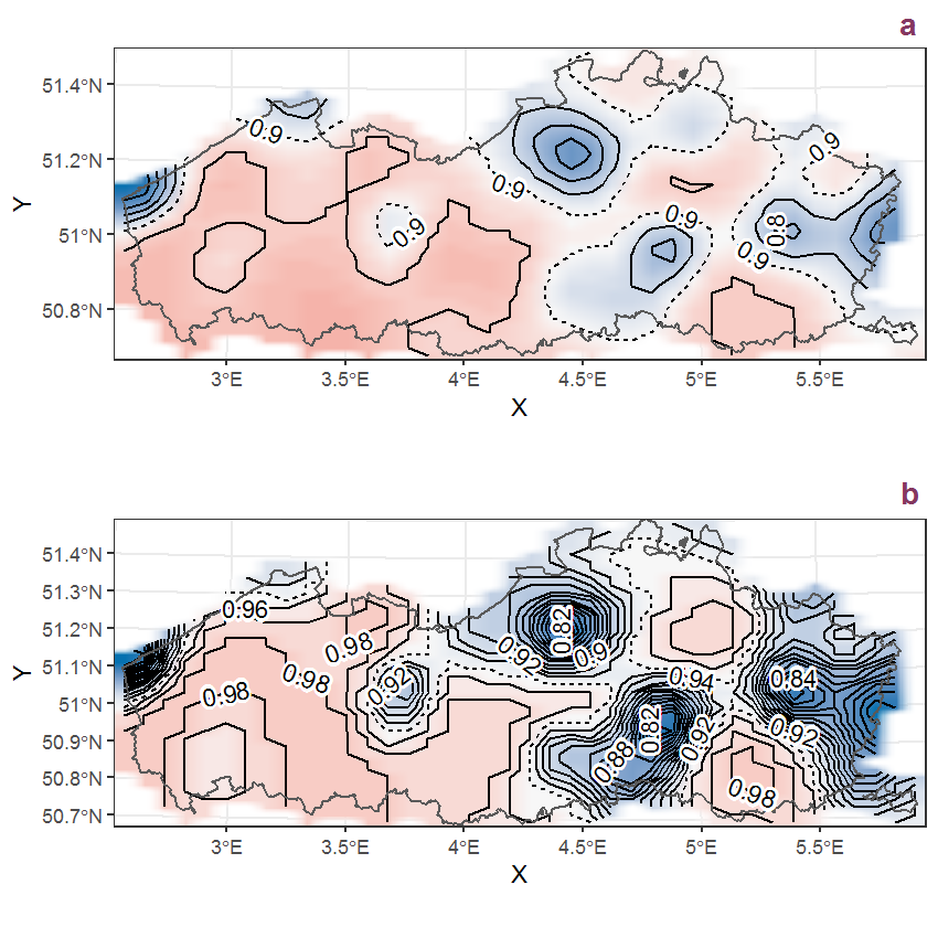
Figure P.87: Visualisation of the spatial smooth effect on the probability of Ranunculus repens L. presence in 1 km x 1 km squares where the species has been observed at least once. The probabilities (values on the contour lines) are conditional on the final year of observation and a list-length equal to 130. The dashed contour line demarcates zones where the species is expected to be more prevalent (red shades) from zones where the species is less prevalent (blue shades). a: 1950 - 2018, b: 1990 - 2018.
P.30 Ranunculus sardous Crantz
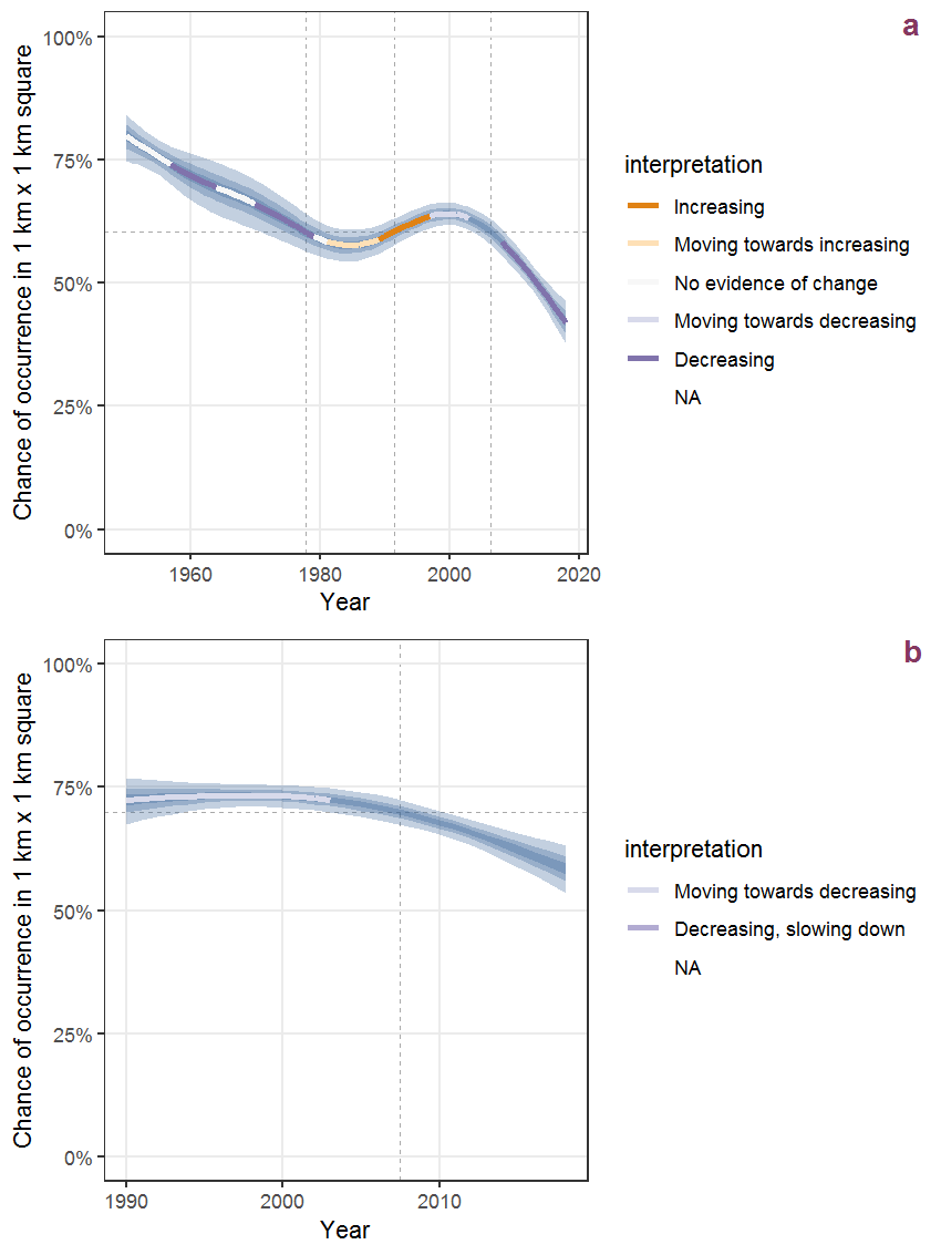
Figure P.88: Effect of year on the probability of Ranunculus sardous Crantz presence in 1 km x 1 km squares where the species has been observed at least once. The fitted line shows the sum of the overall mean (the intercept), a conditional effect of list-length equal to 130 and the year-smoother. The vertical dashed lines indicate the year(s) where the year-smoother is zero. The 95% confidence band is shown in grey (including the variability around the intercept and the smoother). a: 1950 - 2018, b: 1990 - 2018.
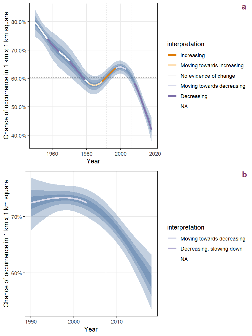
Figure P.89: The same as P.88, but the vertical axis is scaled to the range of the predicted values such that relative changes can be seen more easily. a: 1950 - 2018, b: 1990 - 2018.
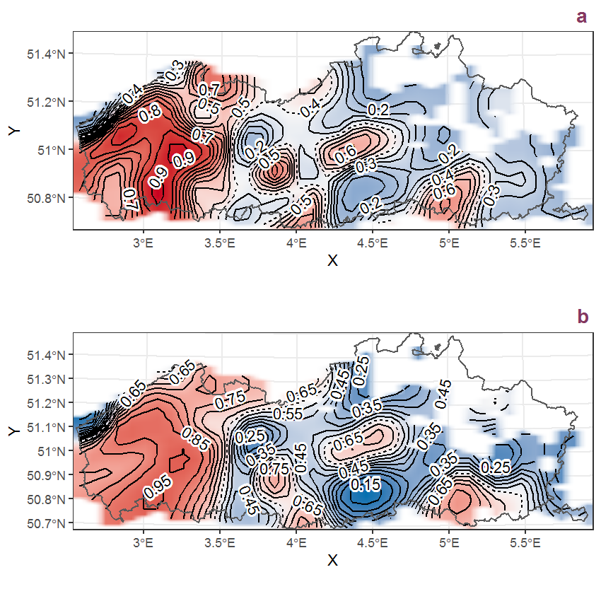
Figure P.90: Visualisation of the spatial smooth effect on the probability of Ranunculus sardous Crantz presence in 1 km x 1 km squares where the species has been observed at least once. The probabilities (values on the contour lines) are conditional on the final year of observation and a list-length equal to 130. The dashed contour line demarcates zones where the species is expected to be more prevalent (red shades) from zones where the species is less prevalent (blue shades). a: 1950 - 2018, b: 1990 - 2018.
P.31 Ranunculus sceleratus L.
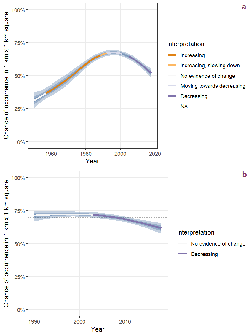
Figure P.91: Effect of year on the probability of Ranunculus sceleratus L. presence in 1 km x 1 km squares where the species has been observed at least once. The fitted line shows the sum of the overall mean (the intercept), a conditional effect of list-length equal to 130 and the year-smoother. The vertical dashed lines indicate the year(s) where the year-smoother is zero. The 95% confidence band is shown in grey (including the variability around the intercept and the smoother). a: 1950 - 2018, b: 1990 - 2018.
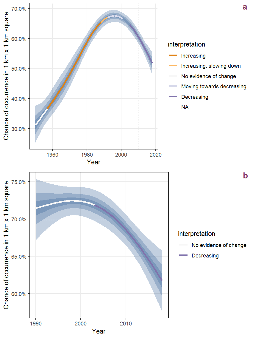
Figure P.92: The same as P.91, but the vertical axis is scaled to the range of the predicted values such that relative changes can be seen more easily. a: 1950 - 2018, b: 1990 - 2018.
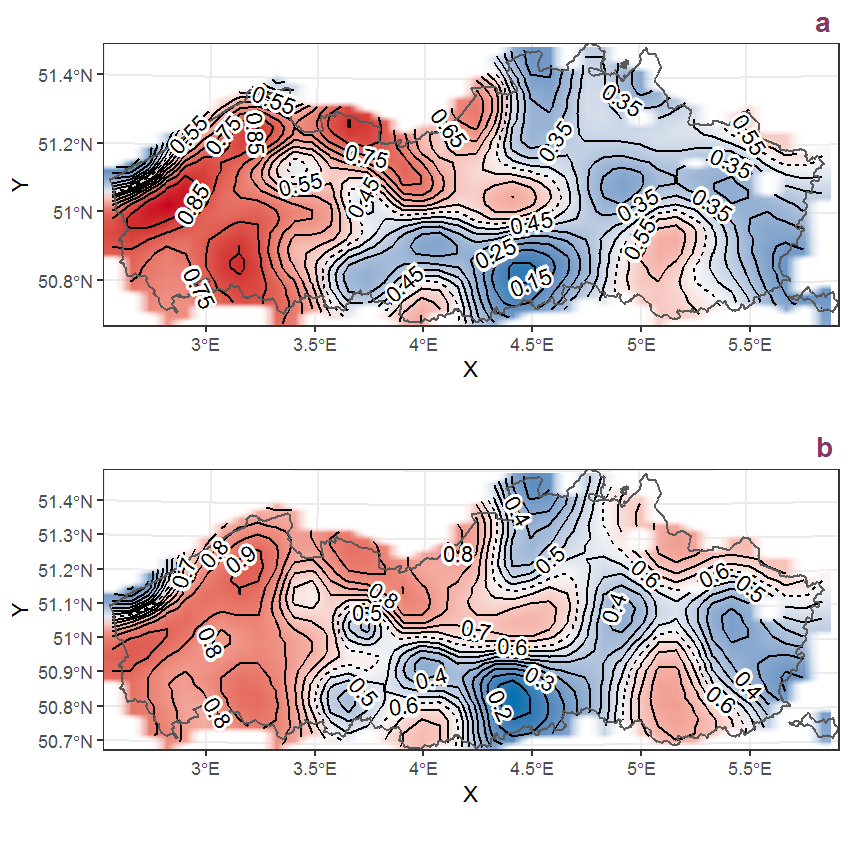
Figure P.93: Visualisation of the spatial smooth effect on the probability of Ranunculus sceleratus L. presence in 1 km x 1 km squares where the species has been observed at least once. The probabilities (values on the contour lines) are conditional on the final year of observation and a list-length equal to 130. The dashed contour line demarcates zones where the species is expected to be more prevalent (red shades) from zones where the species is less prevalent (blue shades). a: 1950 - 2018, b: 1990 - 2018.
P.32 Raphanus raphanistrum L.
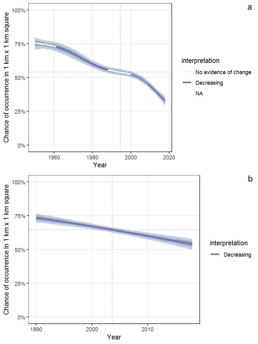
Figure P.94: Effect of year on the probability of Raphanus raphanistrum L. presence in 1 km x 1 km squares where the species has been observed at least once. The fitted line shows the sum of the overall mean (the intercept), a conditional effect of list-length equal to 130 and the year-smoother. The vertical dashed lines indicate the year(s) where the year-smoother is zero. The 95% confidence band is shown in grey (including the variability around the intercept and the smoother). a: 1950 - 2018, b: 1990 - 2018.
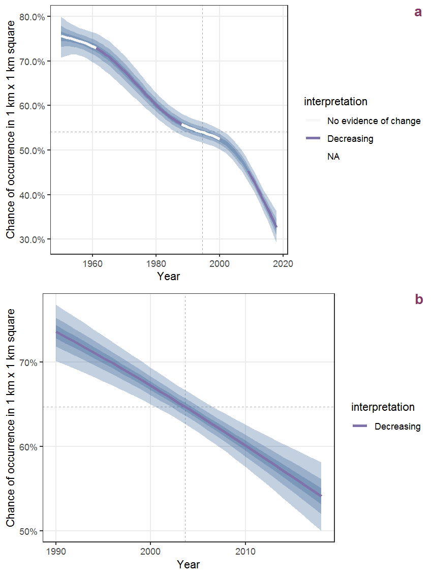
Figure P.95: The same as P.94, but the vertical axis is scaled to the range of the predicted values such that relative changes can be seen more easily. a: 1950 - 2018, b: 1990 - 2018.
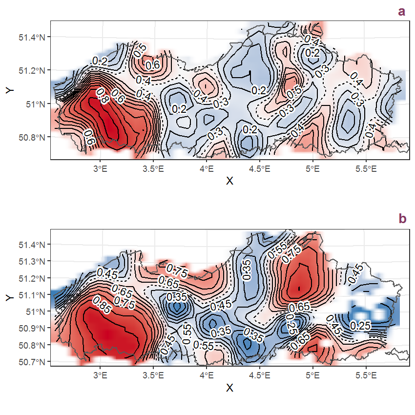
Figure P.96: Visualisation of the spatial smooth effect on the probability of Raphanus raphanistrum L. presence in 1 km x 1 km squares where the species has been observed at least once. The probabilities (values on the contour lines) are conditional on the final year of observation and a list-length equal to 130. The dashed contour line demarcates zones where the species is expected to be more prevalent (red shades) from zones where the species is less prevalent (blue shades). a: 1950 - 2018, b: 1990 - 2018.