B Acer campestre L. - Amaranthus retroflexus L.
B.1 Acer campestre L.
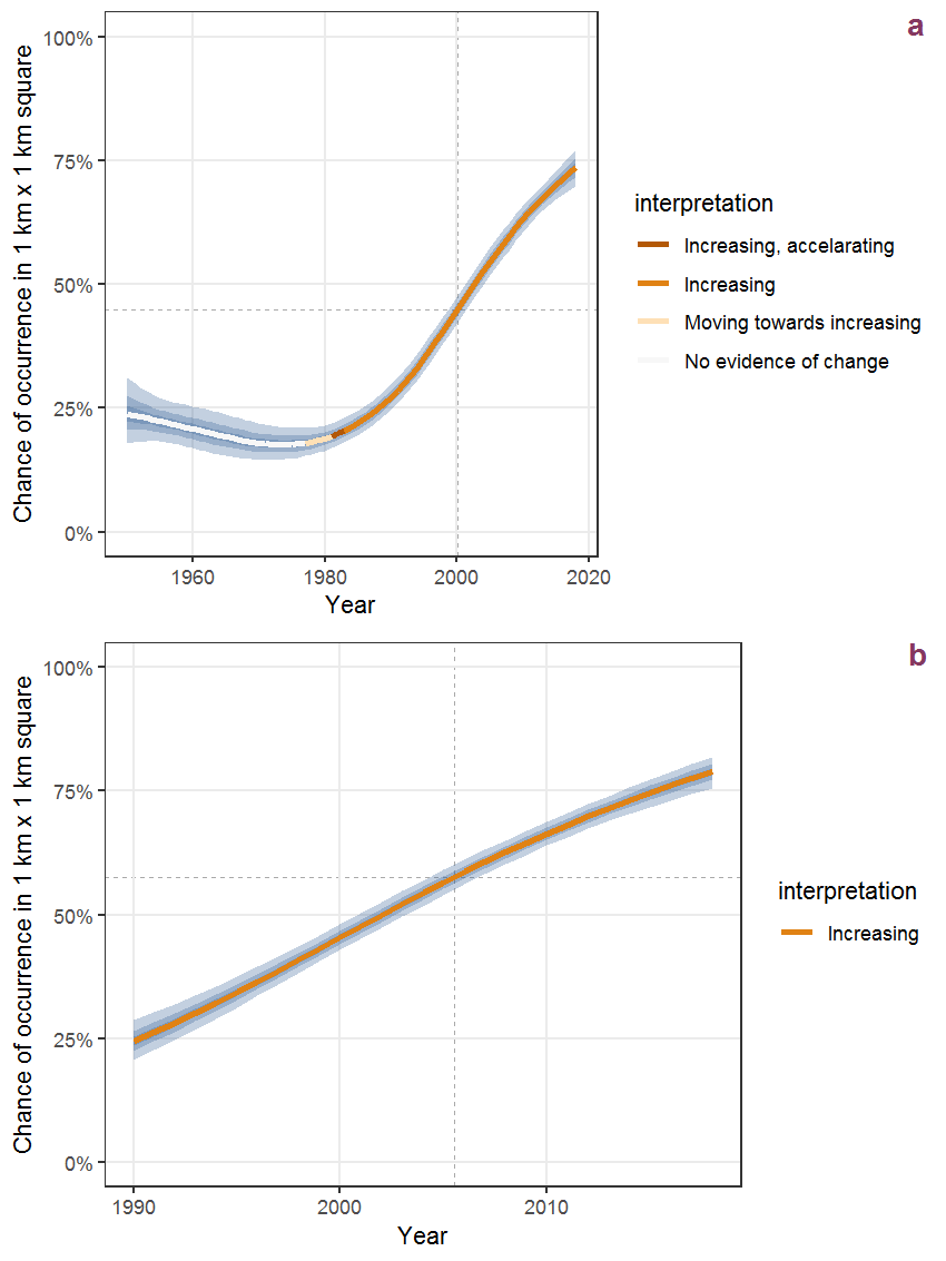
Figure B.1: Effect of year on the probability of Acer campestre L. presence in 1 km x 1 km squares where the species has been observed at least once. The fitted line shows the sum of the overall mean (the intercept), a conditional effect of list-length equal to 130 and the year-smoother. The vertical dashed lines indicate the year(s) where the year-smoother is zero. The 95% confidence band is shown in grey (including the variability around the intercept and the smoother). a: 1950 - 2018, b: 1990 - 2018.
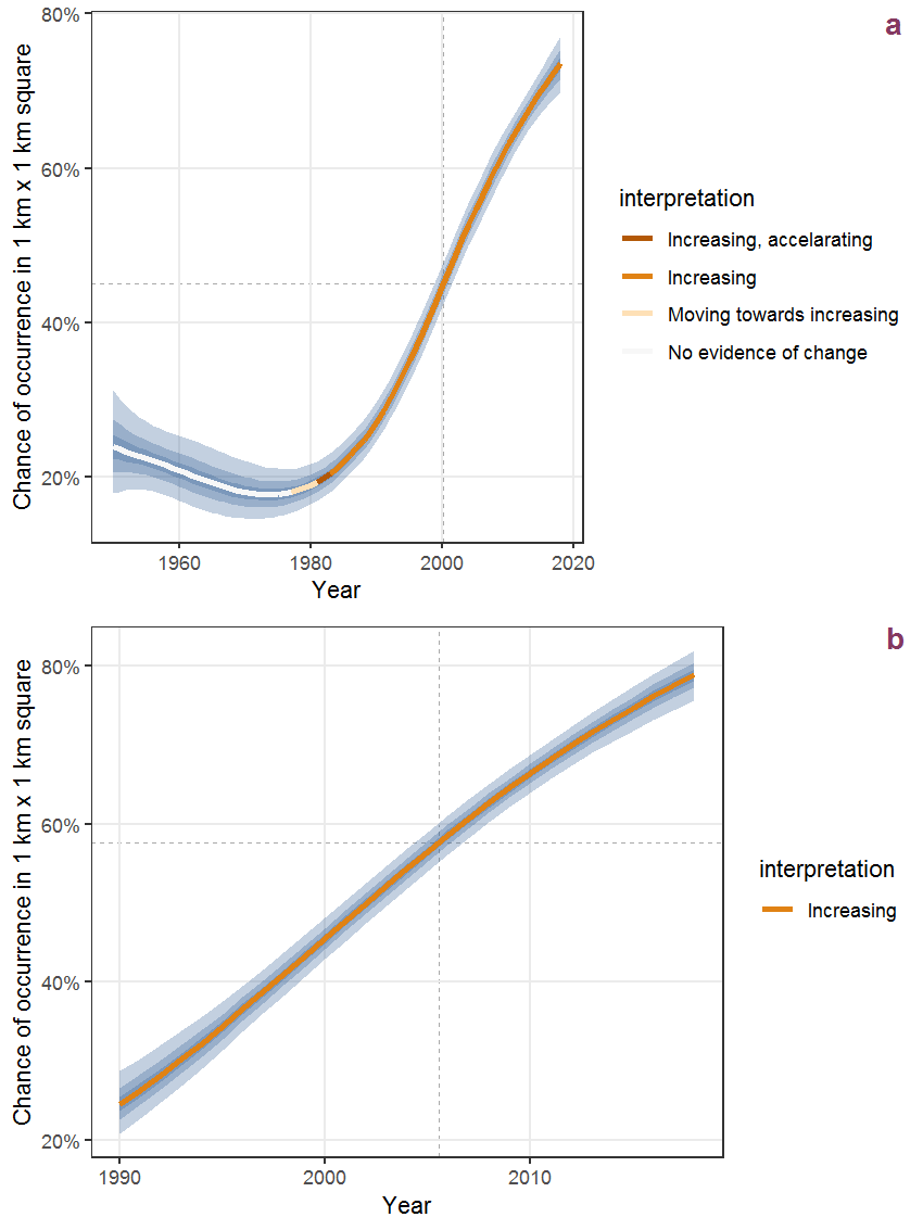
Figure B.2: The same as B.1, but the vertical axis is scaled to the range of the predicted values such that relative changes can be seen more easily. a: 1950 - 2018, b: 1990 - 2018.
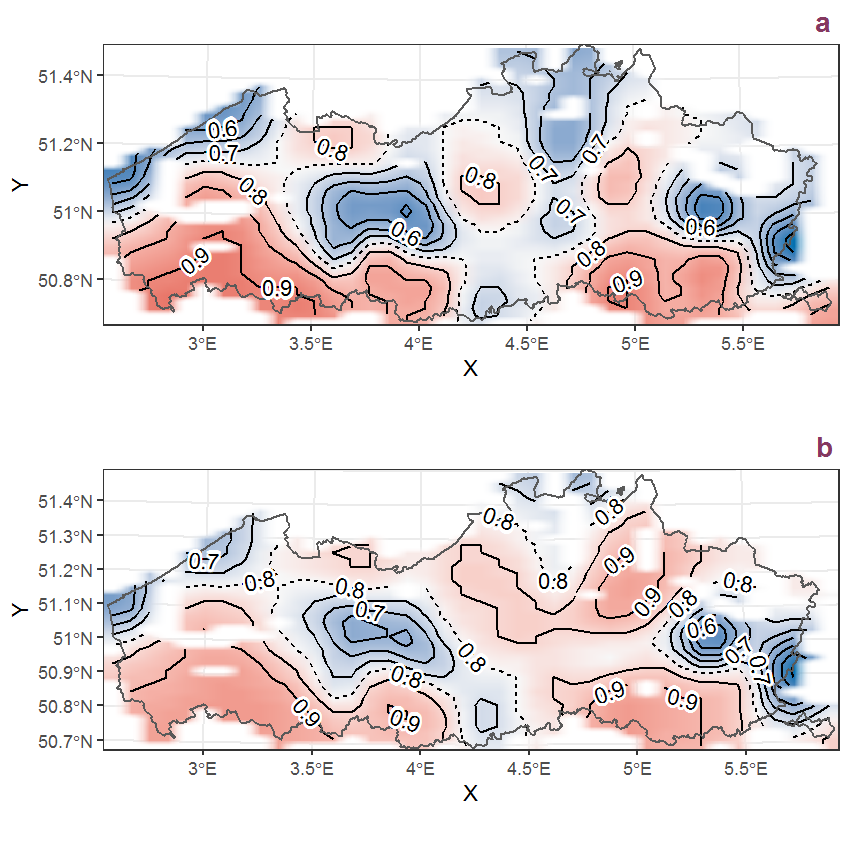
Figure B.3: Visualisation of the spatial smooth effect on the probability of Acer campestre L. presence in 1 km x 1 km squares where the species has been observed at least once. The probabilities (values on the contour lines) are conditional on the final year of observation and a list-length equal to 130. The dashed contour line demarcates zones where the species is expected to be more prevalent (red shades) from zones where the species is less prevalent (blue shades). a: 1950 - 2018, b: 1990 - 2018.
B.2 Acer negundo L.
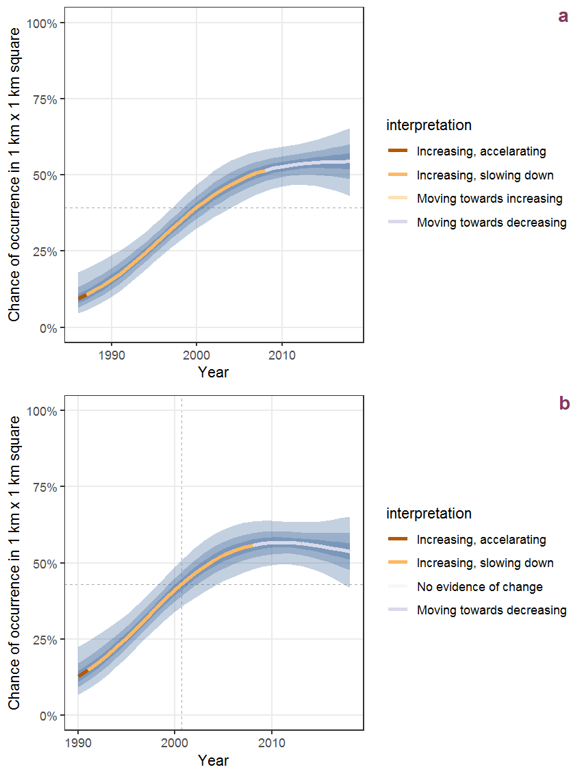
Figure B.4: Effect of year on the probability of Acer negundo L. presence in 1 km x 1 km squares where the species has been observed at least once. The fitted line shows the sum of the overall mean (the intercept), a conditional effect of list-length equal to 130 and the year-smoother. The vertical dashed lines indicate the year(s) where the year-smoother is zero. The 95% confidence band is shown in grey (including the variability around the intercept and the smoother). a: 1950 - 2018, b: 1990 - 2018.
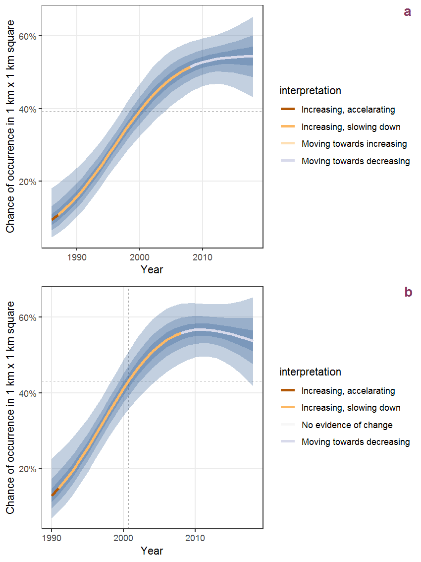
Figure B.5: The same as B.4, but the vertical axis is scaled to the range of the predicted values such that relative changes can be seen more easily. a: 1950 - 2018, b: 1990 - 2018.
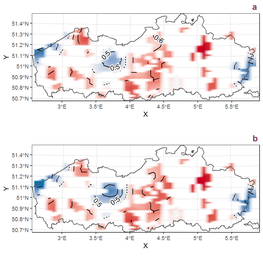
Figure B.6: Visualisation of the spatial smooth effect on the probability of Acer negundo L. presence in 1 km x 1 km squares where the species has been observed at least once. The probabilities (values on the contour lines) are conditional on the final year of observation and a list-length equal to 130. The dashed contour line demarcates zones where the species is expected to be more prevalent (red shades) from zones where the species is less prevalent (blue shades). a: 1950 - 2018, b: 1990 - 2018.
B.3 Acer platanoides L.
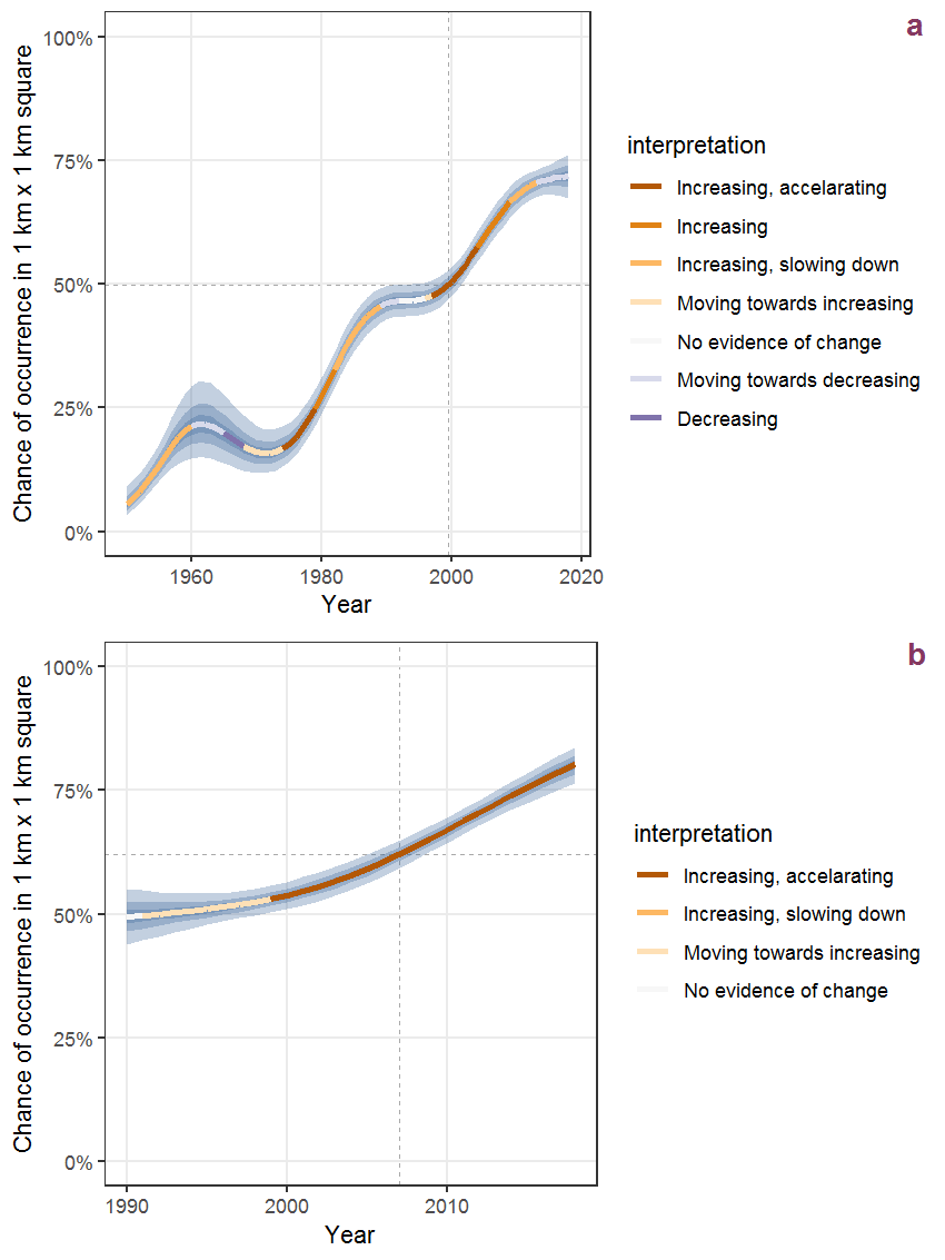
Figure B.7: Effect of year on the probability of Acer platanoides L. presence in 1 km x 1 km squares where the species has been observed at least once. The fitted line shows the sum of the overall mean (the intercept), a conditional effect of list-length equal to 130 and the year-smoother. The vertical dashed lines indicate the year(s) where the year-smoother is zero. The 95% confidence band is shown in grey (including the variability around the intercept and the smoother). a: 1950 - 2018, b: 1990 - 2018.
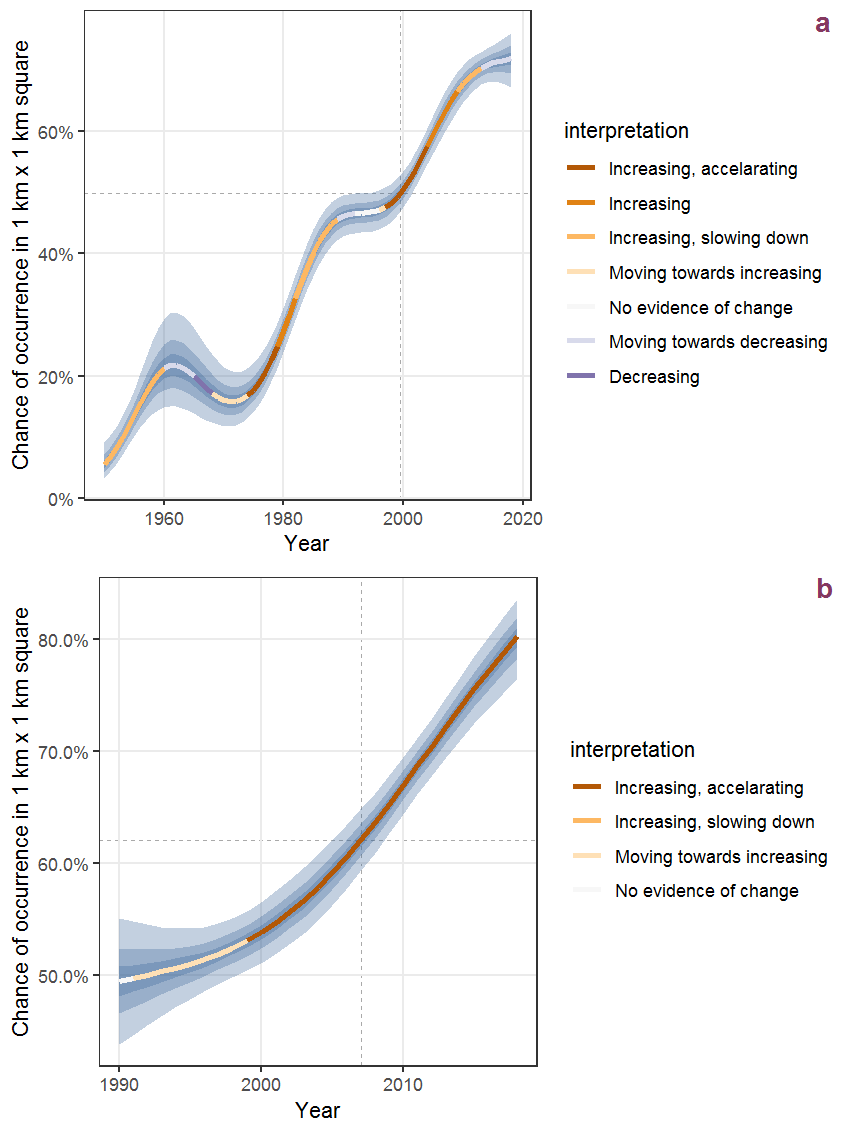
Figure B.8: The same as B.7, but the vertical axis is scaled to the range of the predicted values such that relative changes can be seen more easily. a: 1950 - 2018, b: 1990 - 2018.
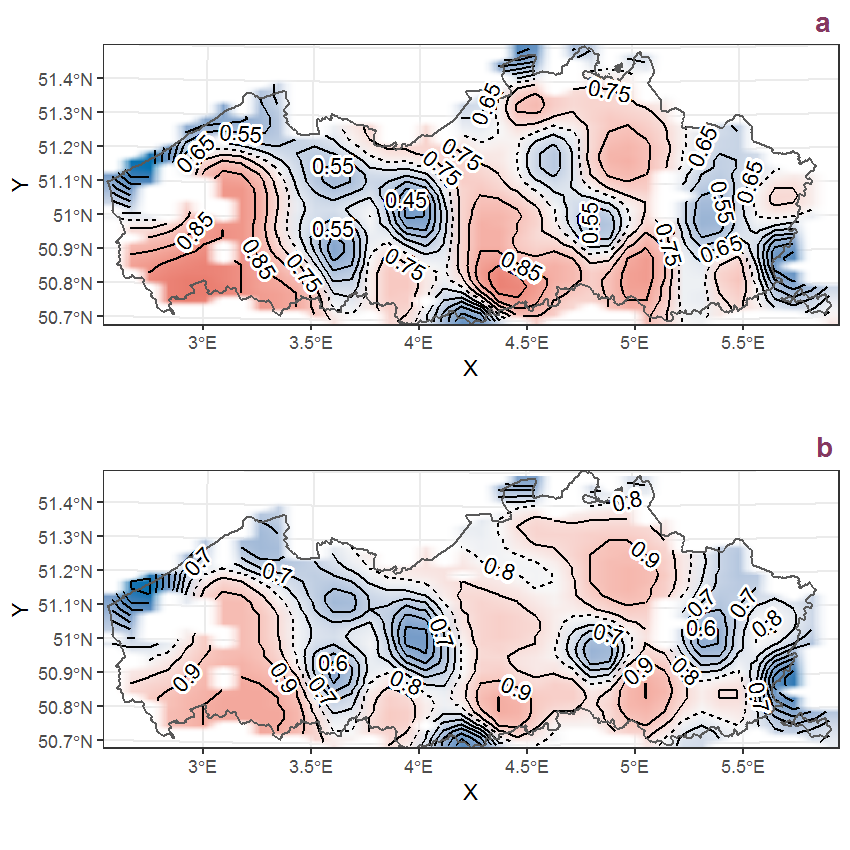
Figure B.9: Visualisation of the spatial smooth effect on the probability of Acer platanoides L. presence in 1 km x 1 km squares where the species has been observed at least once. The probabilities (values on the contour lines) are conditional on the final year of observation and a list-length equal to 130. The dashed contour line demarcates zones where the species is expected to be more prevalent (red shades) from zones where the species is less prevalent (blue shades). a: 1950 - 2018, b: 1990 - 2018.
B.4 Acer pseudoplatanus L.
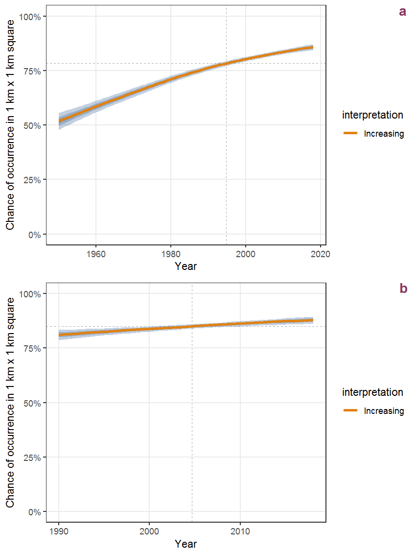
Figure B.10: Effect of year on the probability of Acer pseudoplatanus L. presence in 1 km x 1 km squares where the species has been observed at least once. The fitted line shows the sum of the overall mean (the intercept), a conditional effect of list-length equal to 130 and the year-smoother. The vertical dashed lines indicate the year(s) where the year-smoother is zero. The 95% confidence band is shown in grey (including the variability around the intercept and the smoother). a: 1950 - 2018, b: 1990 - 2018.
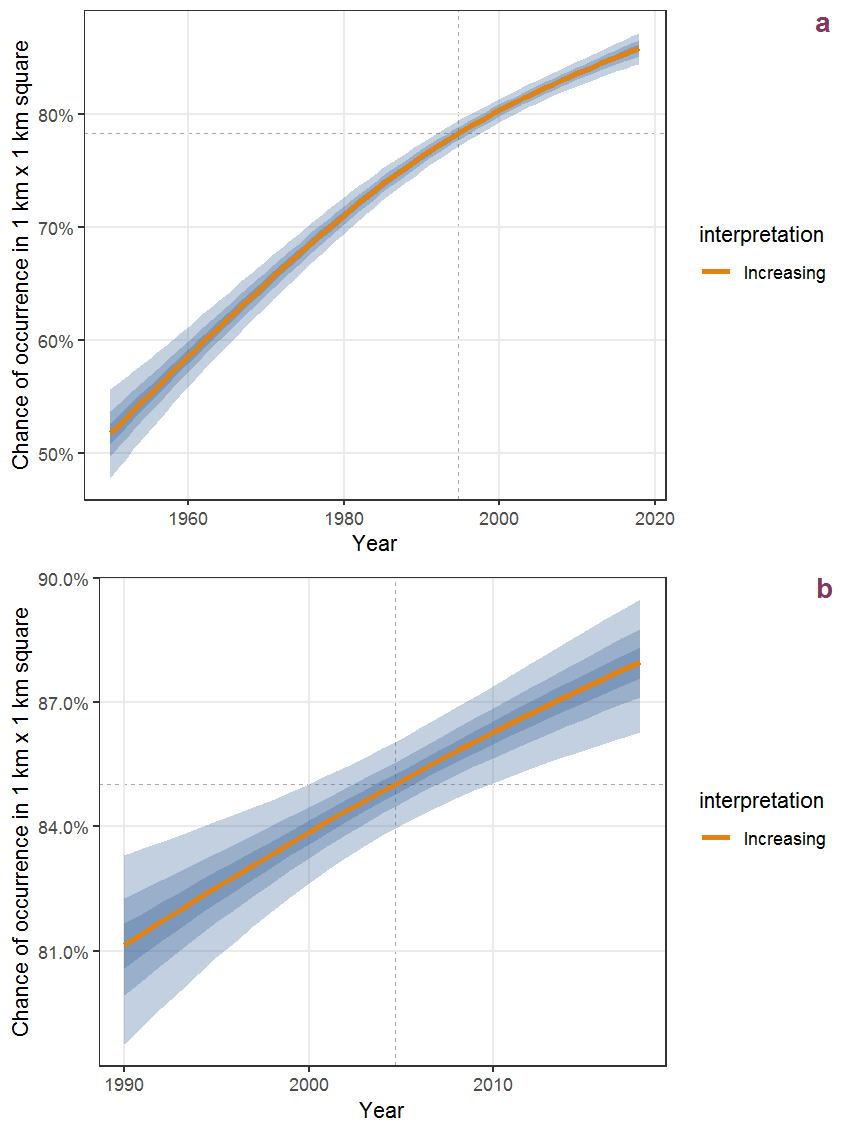
Figure B.11: The same as B.10, but the vertical axis is scaled to the range of the predicted values such that relative changes can be seen more easily. a: 1950 - 2018, b: 1990 - 2018.
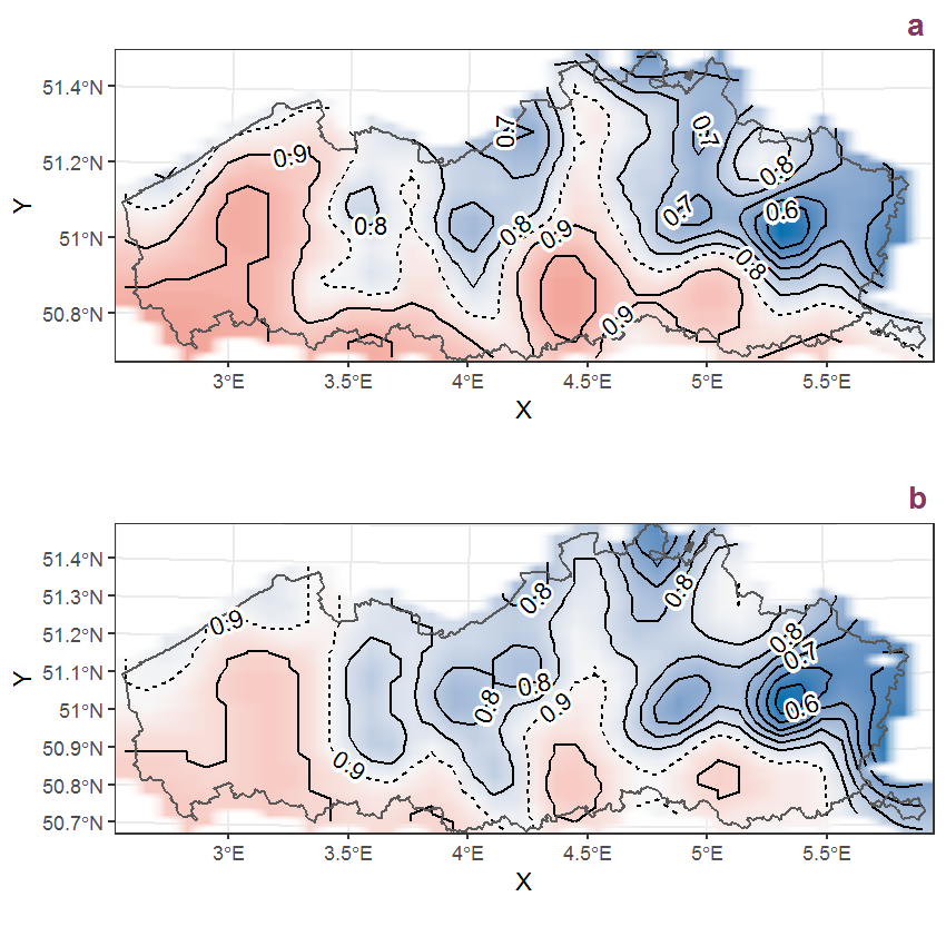
Figure B.12: Visualisation of the spatial smooth effect on the probability of Acer pseudoplatanus L. presence in 1 km x 1 km squares where the species has been observed at least once. The probabilities (values on the contour lines) are conditional on the final year of observation and a list-length equal to 130. The dashed contour line demarcates zones where the species is expected to be more prevalent (red shades) from zones where the species is less prevalent (blue shades). a: 1950 - 2018, b: 1990 - 2018.
B.5 Achillea millefolium L.
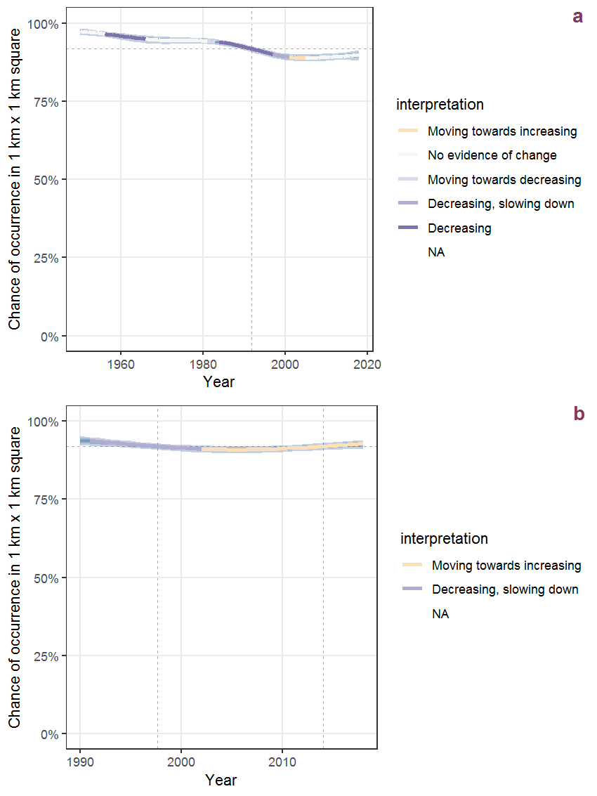
Figure B.13: Effect of year on the probability of Achillea millefolium L. presence in 1 km x 1 km squares where the species has been observed at least once. The fitted line shows the sum of the overall mean (the intercept), a conditional effect of list-length equal to 130 and the year-smoother. The vertical dashed lines indicate the year(s) where the year-smoother is zero. The 95% confidence band is shown in grey (including the variability around the intercept and the smoother). a: 1950 - 2018, b: 1990 - 2018.
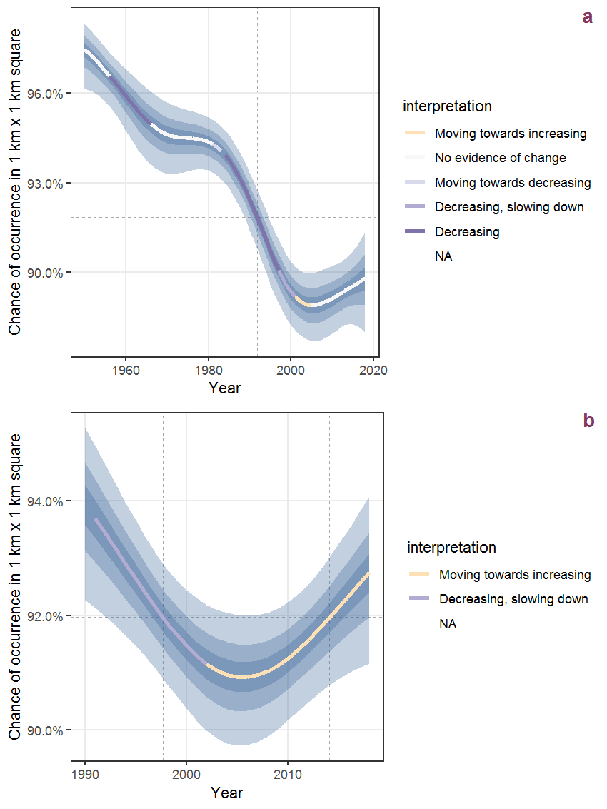
Figure B.14: The same as B.13, but the vertical axis is scaled to the range of the predicted values such that relative changes can be seen more easily. a: 1950 - 2018, b: 1990 - 2018.
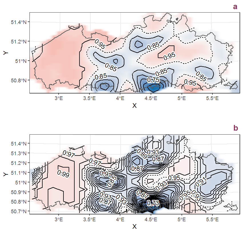
Figure B.15: Visualisation of the spatial smooth effect on the probability of Achillea millefolium L. presence in 1 km x 1 km squares where the species has been observed at least once. The probabilities (values on the contour lines) are conditional on the final year of observation and a list-length equal to 130. The dashed contour line demarcates zones where the species is expected to be more prevalent (red shades) from zones where the species is less prevalent (blue shades). a: 1950 - 2018, b: 1990 - 2018.
B.6 Achillea ptarmica L.
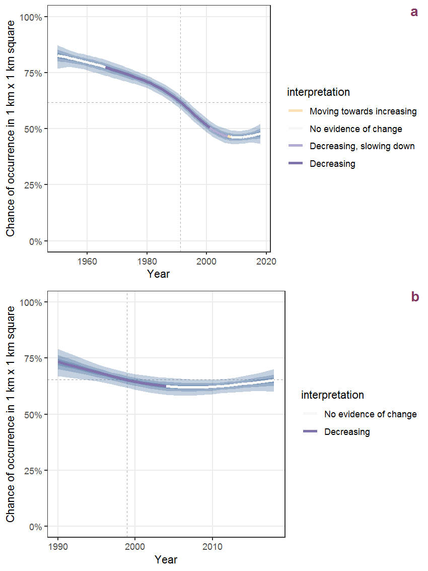
Figure B.16: Effect of year on the probability of Achillea ptarmica L. presence in 1 km x 1 km squares where the species has been observed at least once. The fitted line shows the sum of the overall mean (the intercept), a conditional effect of list-length equal to 130 and the year-smoother. The vertical dashed lines indicate the year(s) where the year-smoother is zero. The 95% confidence band is shown in grey (including the variability around the intercept and the smoother). a: 1950 - 2018, b: 1990 - 2018.
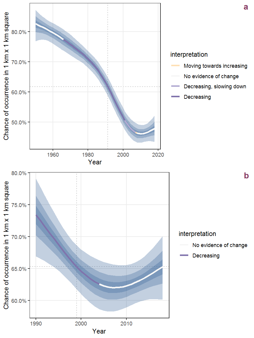
Figure B.17: The same as B.16, but the vertical axis is scaled to the range of the predicted values such that relative changes can be seen more easily. a: 1950 - 2018, b: 1990 - 2018.
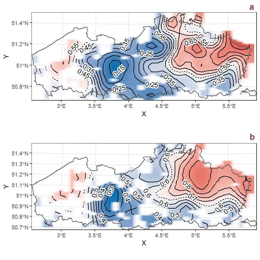
Figure B.18: Visualisation of the spatial smooth effect on the probability of Achillea ptarmica L. presence in 1 km x 1 km squares where the species has been observed at least once. The probabilities (values on the contour lines) are conditional on the final year of observation and a list-length equal to 130. The dashed contour line demarcates zones where the species is expected to be more prevalent (red shades) from zones where the species is less prevalent (blue shades). a: 1950 - 2018, b: 1990 - 2018.
B.7 Acorus calamus L.
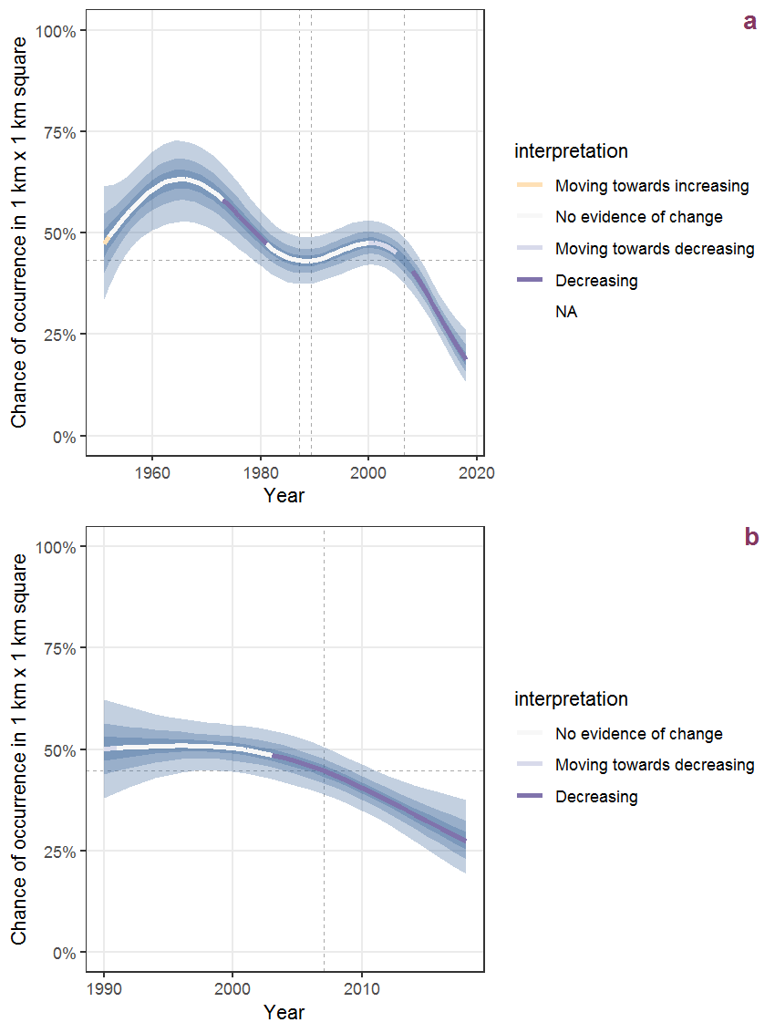
Figure B.19: Effect of year on the probability of Acorus calamus L. presence in 1 km x 1 km squares where the species has been observed at least once. The fitted line shows the sum of the overall mean (the intercept), a conditional effect of list-length equal to 130 and the year-smoother. The vertical dashed lines indicate the year(s) where the year-smoother is zero. The 95% confidence band is shown in grey (including the variability around the intercept and the smoother). a: 1950 - 2018, b: 1990 - 2018.
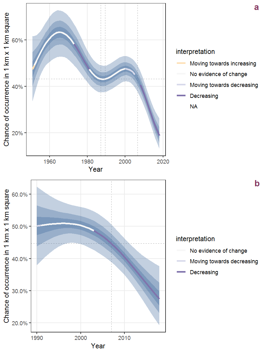
Figure B.20: The same as B.19, but the vertical axis is scaled to the range of the predicted values such that relative changes can be seen more easily. a: 1950 - 2018, b: 1990 - 2018.
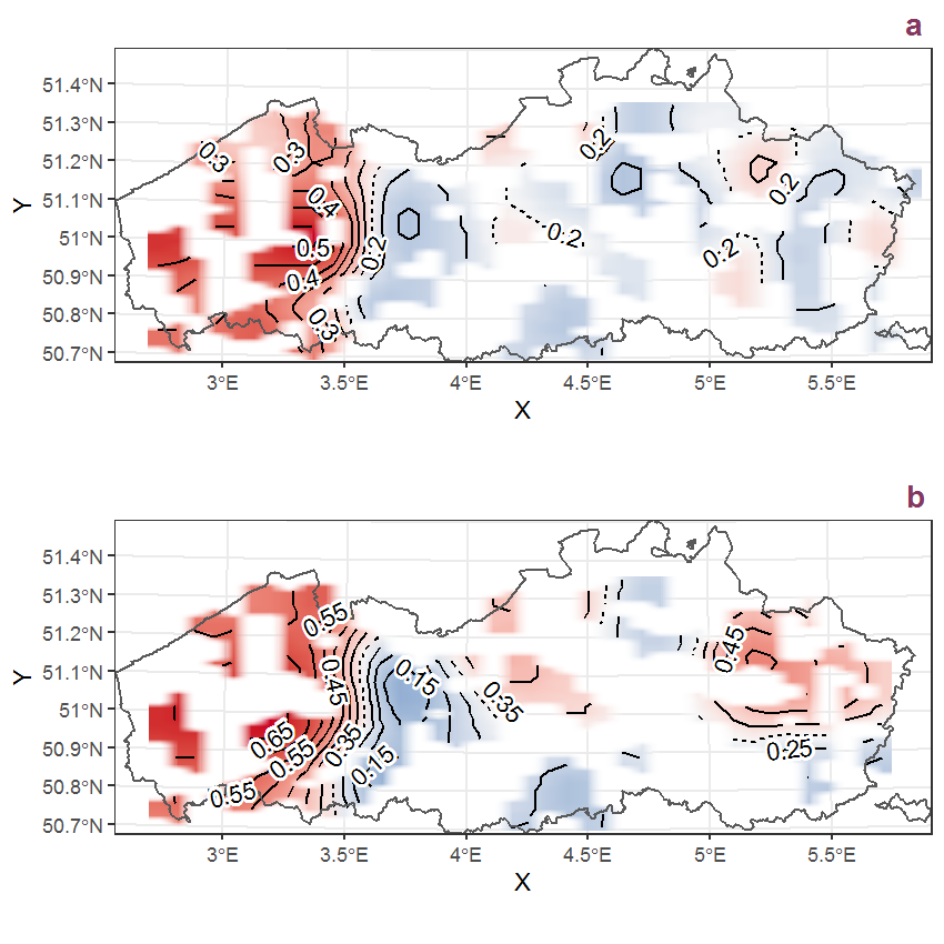
Figure B.21: Visualisation of the spatial smooth effect on the probability of Acorus calamus L. presence in 1 km x 1 km squares where the species has been observed at least once. The probabilities (values on the contour lines) are conditional on the final year of observation and a list-length equal to 130. The dashed contour line demarcates zones where the species is expected to be more prevalent (red shades) from zones where the species is less prevalent (blue shades). a: 1950 - 2018, b: 1990 - 2018.
B.8 Adoxa moschatellina L.
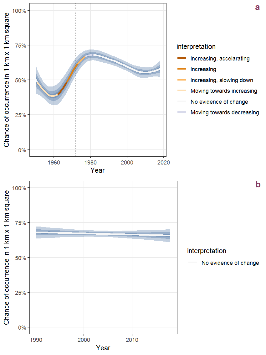
Figure B.22: Effect of year on the probability of Adoxa moschatellina L. presence in 1 km x 1 km squares where the species has been observed at least once. The fitted line shows the sum of the overall mean (the intercept), a conditional effect of list-length equal to 130 and the year-smoother. The vertical dashed lines indicate the year(s) where the year-smoother is zero. The 95% confidence band is shown in grey (including the variability around the intercept and the smoother). a: 1950 - 2018, b: 1990 - 2018.
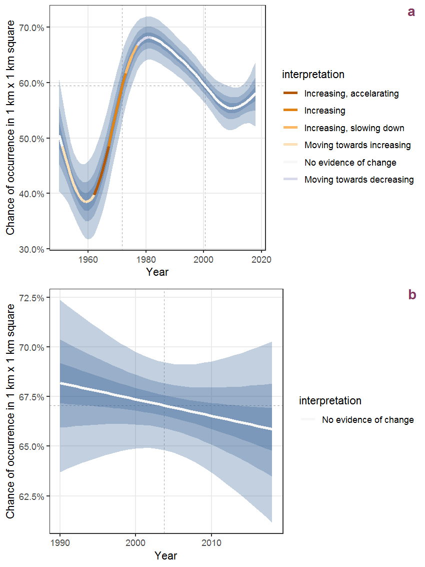
Figure B.23: The same as B.22, but the vertical axis is scaled to the range of the predicted values such that relative changes can be seen more easily. a: 1950 - 2018, b: 1990 - 2018.
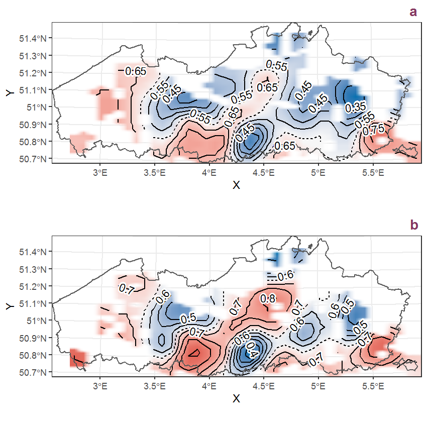
Figure B.24: Visualisation of the spatial smooth effect on the probability of Adoxa moschatellina L. presence in 1 km x 1 km squares where the species has been observed at least once. The probabilities (values on the contour lines) are conditional on the final year of observation and a list-length equal to 130. The dashed contour line demarcates zones where the species is expected to be more prevalent (red shades) from zones where the species is less prevalent (blue shades). a: 1950 - 2018, b: 1990 - 2018.
B.9 Aegopodium podagraria L.
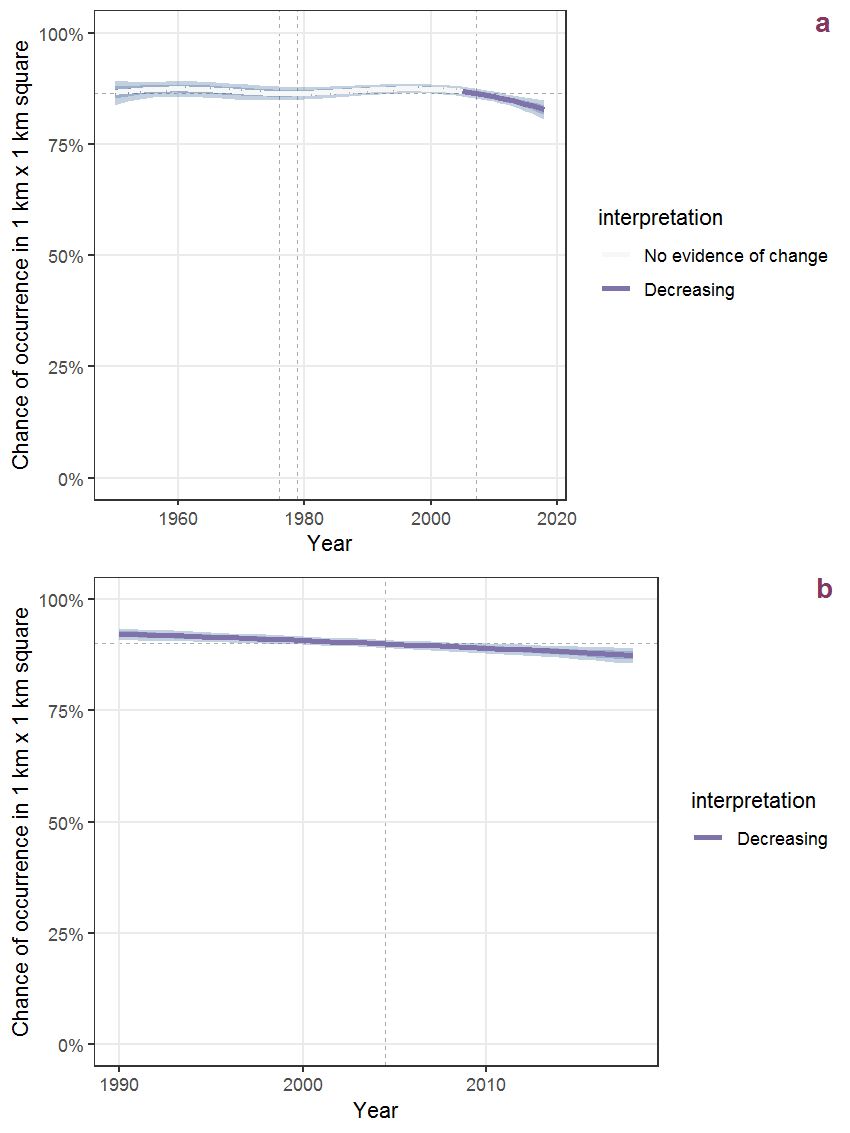
Figure B.25: Effect of year on the probability of Aegopodium podagraria L. presence in 1 km x 1 km squares where the species has been observed at least once. The fitted line shows the sum of the overall mean (the intercept), a conditional effect of list-length equal to 130 and the year-smoother. The vertical dashed lines indicate the year(s) where the year-smoother is zero. The 95% confidence band is shown in grey (including the variability around the intercept and the smoother). a: 1950 - 2018, b: 1990 - 2018.
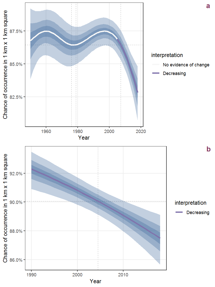
Figure B.26: The same as B.25, but the vertical axis is scaled to the range of the predicted values such that relative changes can be seen more easily. a: 1950 - 2018, b: 1990 - 2018.
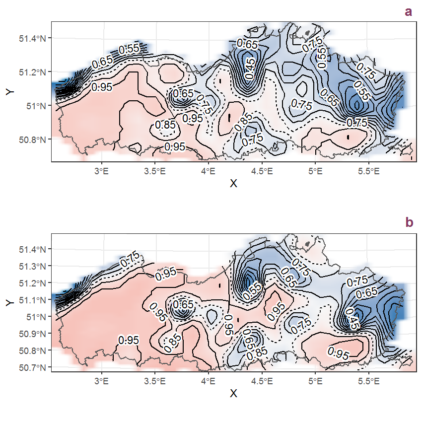
Figure B.27: Visualisation of the spatial smooth effect on the probability of Aegopodium podagraria L. presence in 1 km x 1 km squares where the species has been observed at least once. The probabilities (values on the contour lines) are conditional on the final year of observation and a list-length equal to 130. The dashed contour line demarcates zones where the species is expected to be more prevalent (red shades) from zones where the species is less prevalent (blue shades). a: 1950 - 2018, b: 1990 - 2018.
B.10 Aesculus hippocastanum L.
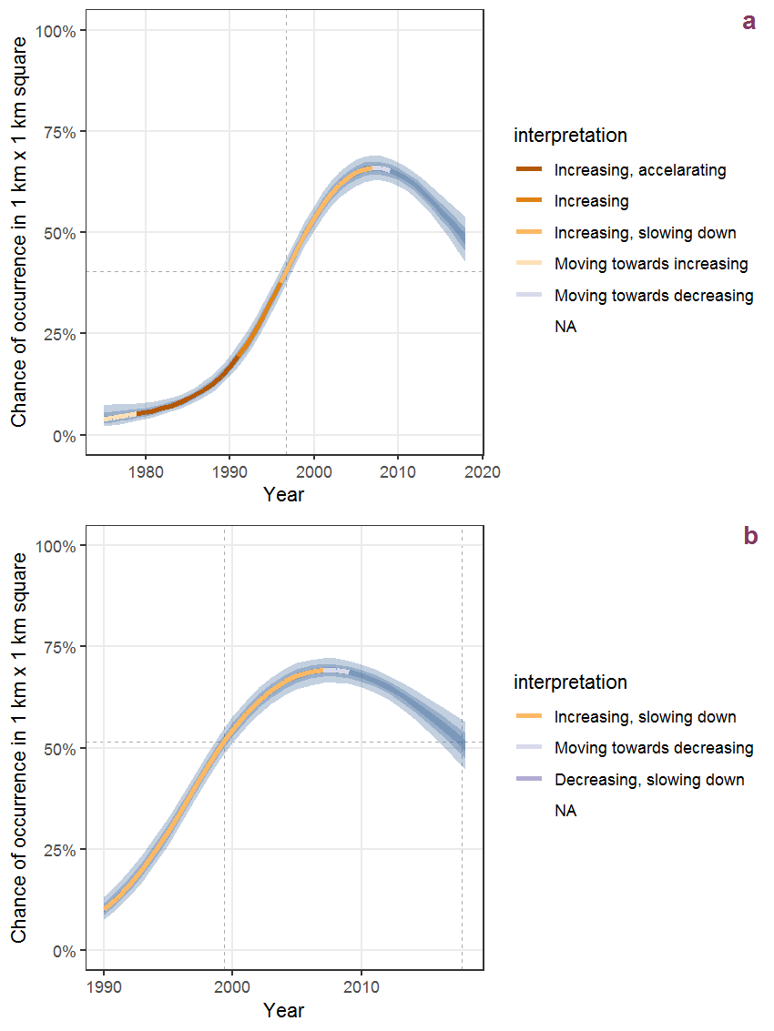
Figure B.28: Effect of year on the probability of Aesculus hippocastanum L. presence in 1 km x 1 km squares where the species has been observed at least once. The fitted line shows the sum of the overall mean (the intercept), a conditional effect of list-length equal to 130 and the year-smoother. The vertical dashed lines indicate the year(s) where the year-smoother is zero. The 95% confidence band is shown in grey (including the variability around the intercept and the smoother). a: 1950 - 2018, b: 1990 - 2018.
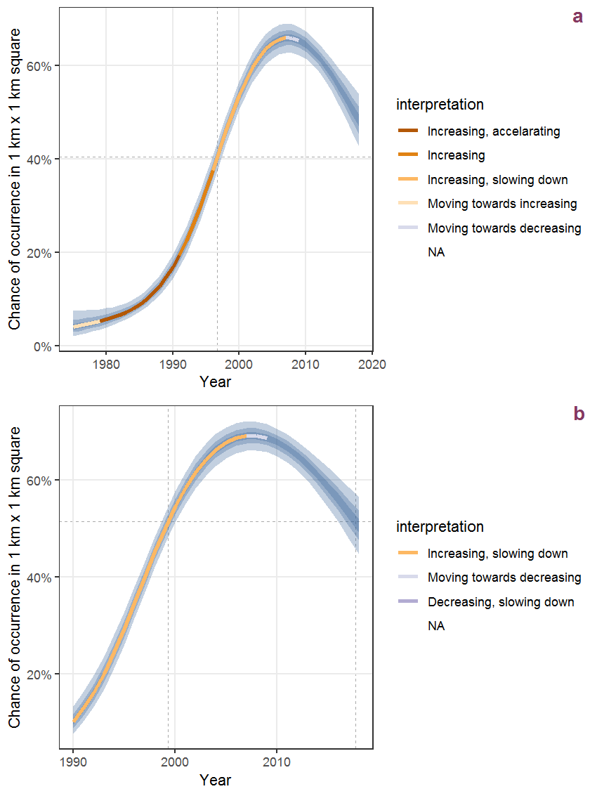
Figure B.29: The same as B.28, but the vertical axis is scaled to the range of the predicted values such that relative changes can be seen more easily. a: 1950 - 2018, b: 1990 - 2018.
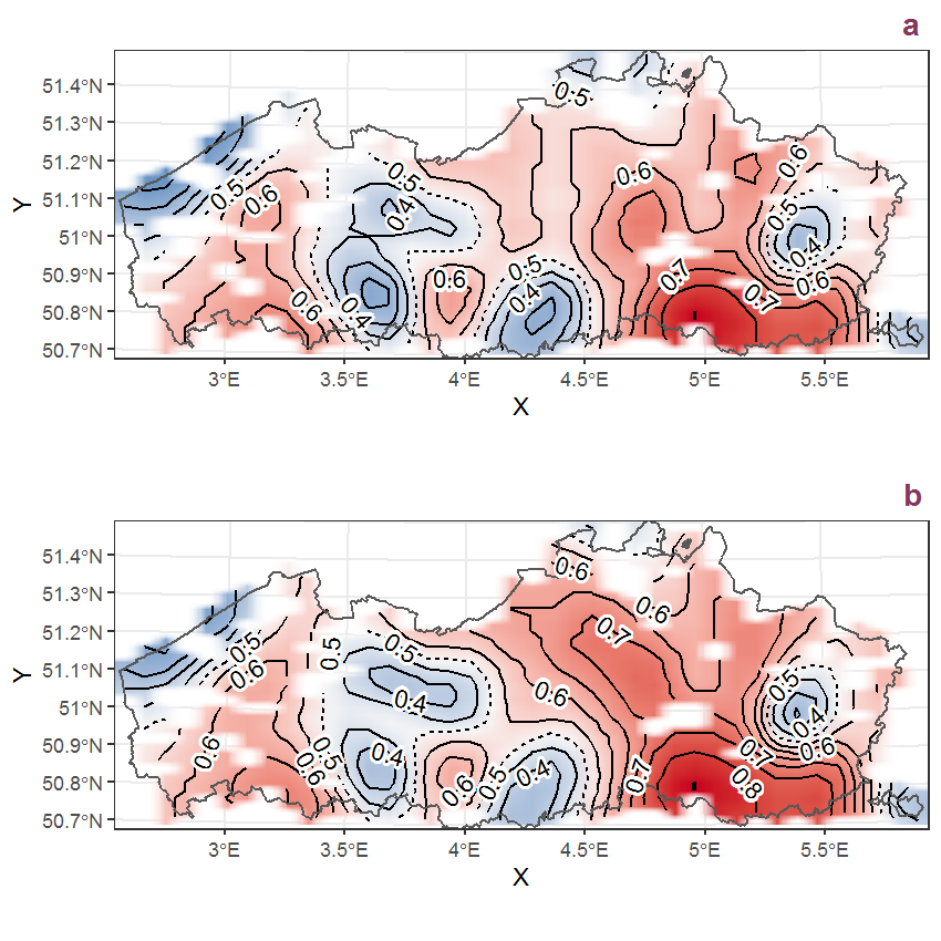
Figure B.30: Visualisation of the spatial smooth effect on the probability of Aesculus hippocastanum L. presence in 1 km x 1 km squares where the species has been observed at least once. The probabilities (values on the contour lines) are conditional on the final year of observation and a list-length equal to 130. The dashed contour line demarcates zones where the species is expected to be more prevalent (red shades) from zones where the species is less prevalent (blue shades). a: 1950 - 2018, b: 1990 - 2018.
B.11 Aethusa cynapium L.
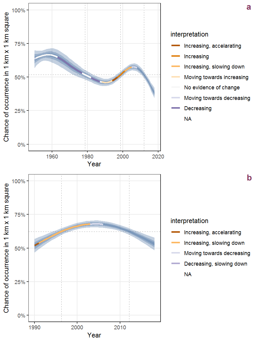
Figure B.31: Effect of year on the probability of Aethusa cynapium L. presence in 1 km x 1 km squares where the species has been observed at least once. The fitted line shows the sum of the overall mean (the intercept), a conditional effect of list-length equal to 130 and the year-smoother. The vertical dashed lines indicate the year(s) where the year-smoother is zero. The 95% confidence band is shown in grey (including the variability around the intercept and the smoother). a: 1950 - 2018, b: 1990 - 2018.
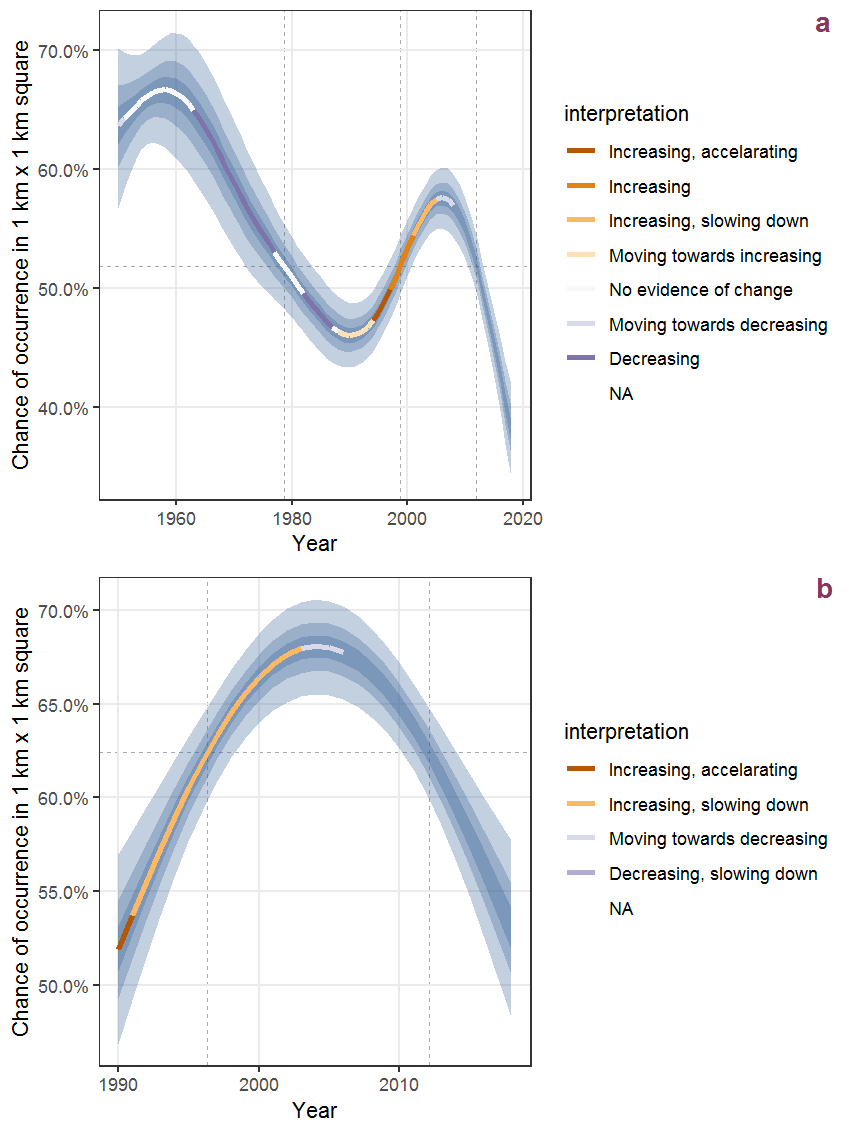
Figure B.32: The same as B.31, but the vertical axis is scaled to the range of the predicted values such that relative changes can be seen more easily. a: 1950 - 2018, b: 1990 - 2018.
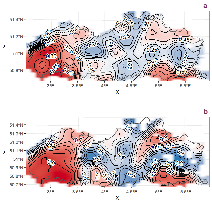
Figure B.33: Visualisation of the spatial smooth effect on the probability of Aethusa cynapium L. presence in 1 km x 1 km squares where the species has been observed at least once. The probabilities (values on the contour lines) are conditional on the final year of observation and a list-length equal to 130. The dashed contour line demarcates zones where the species is expected to be more prevalent (red shades) from zones where the species is less prevalent (blue shades). a: 1950 - 2018, b: 1990 - 2018.
B.12 Agrimonia eupatoria L.
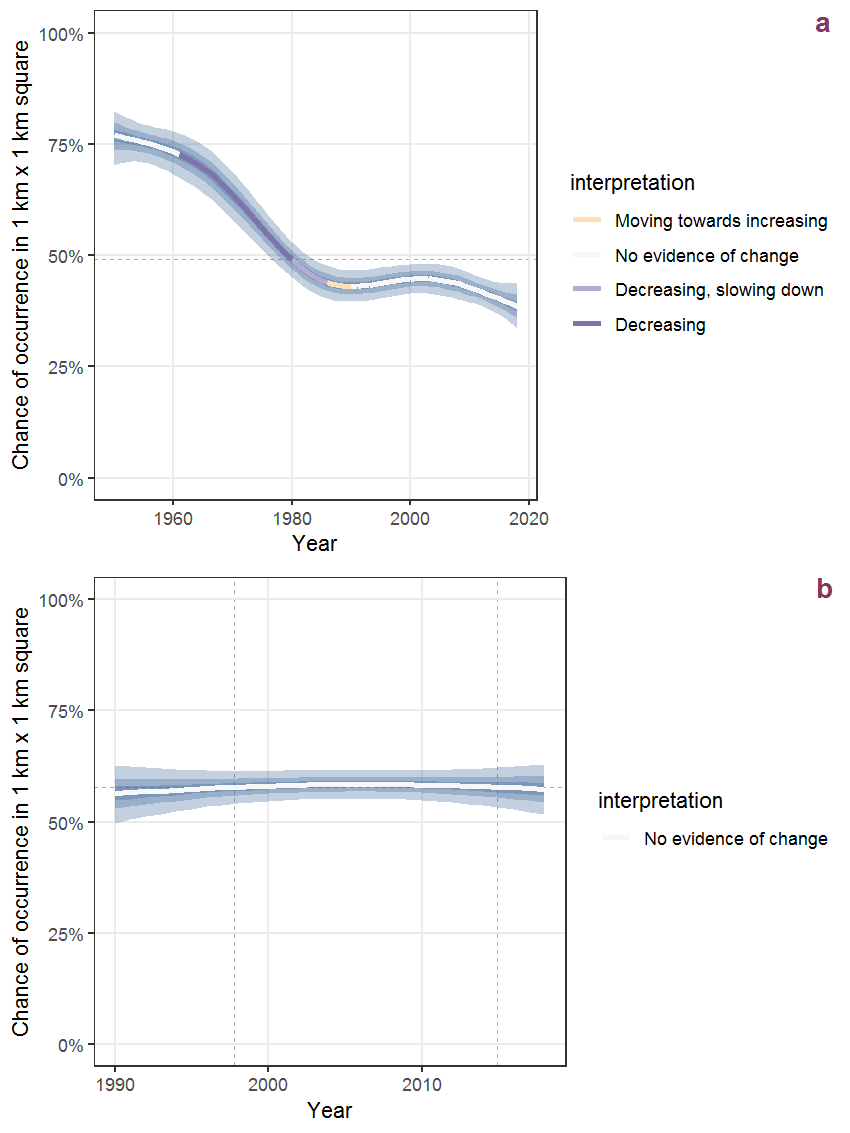
Figure B.34: Effect of year on the probability of Agrimonia eupatoria L. presence in 1 km x 1 km squares where the species has been observed at least once. The fitted line shows the sum of the overall mean (the intercept), a conditional effect of list-length equal to 130 and the year-smoother. The vertical dashed lines indicate the year(s) where the year-smoother is zero. The 95% confidence band is shown in grey (including the variability around the intercept and the smoother). a: 1950 - 2018, b: 1990 - 2018.
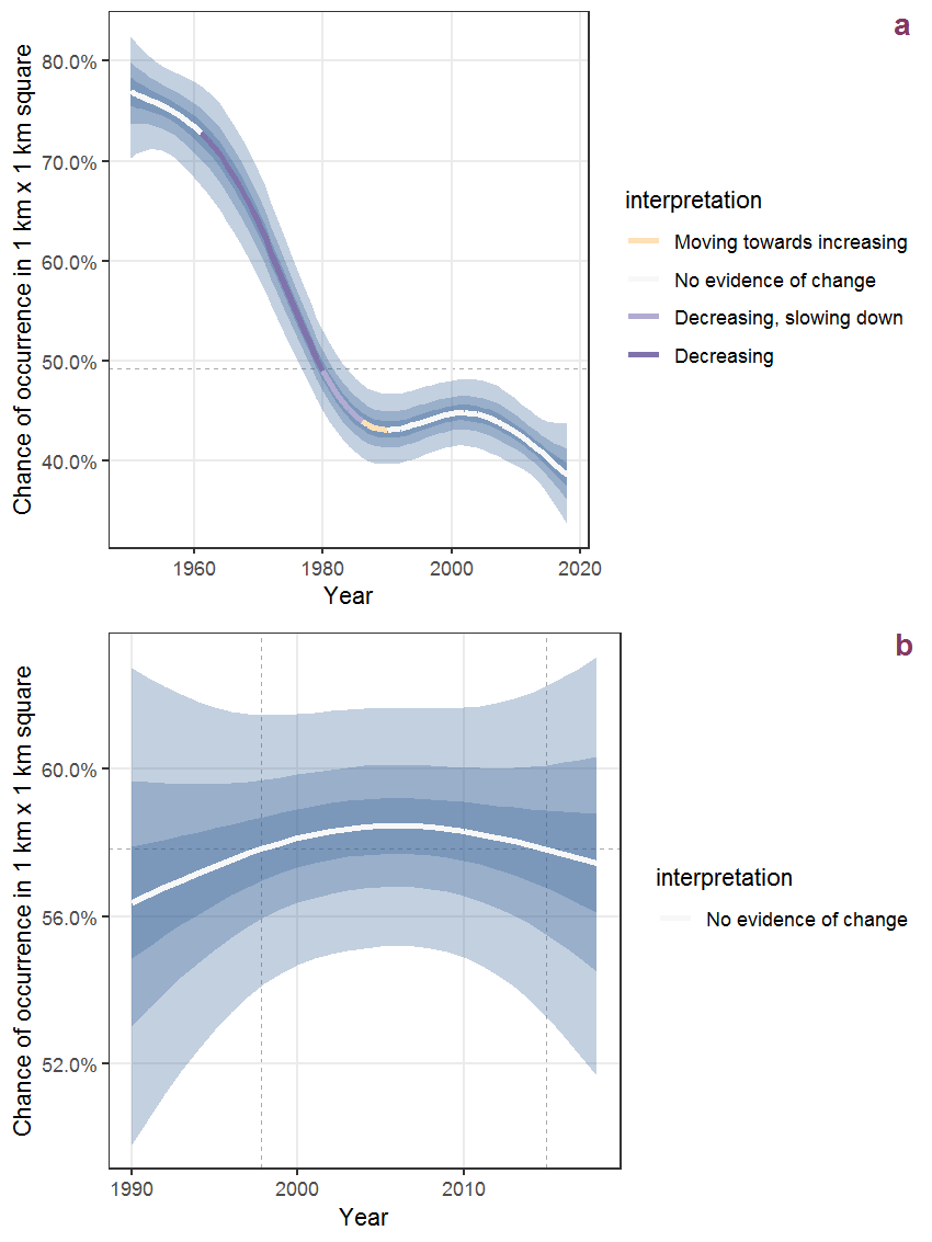
Figure B.35: The same as B.34, but the vertical axis is scaled to the range of the predicted values such that relative changes can be seen more easily. a: 1950 - 2018, b: 1990 - 2018.
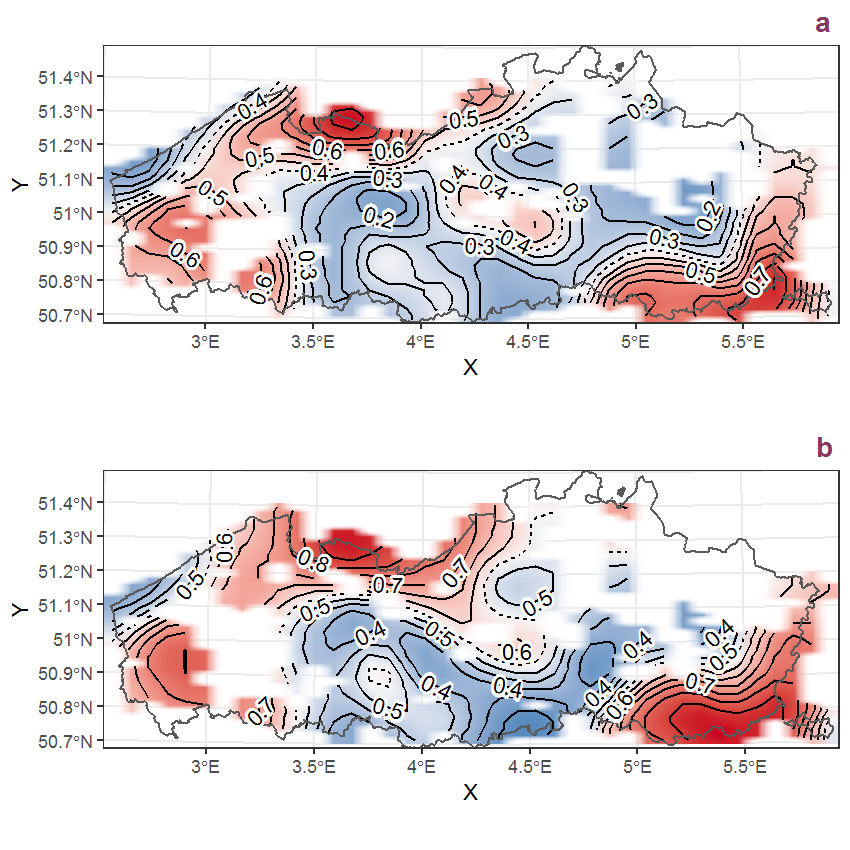
Figure B.36: Visualisation of the spatial smooth effect on the probability of Agrimonia eupatoria L. presence in 1 km x 1 km squares where the species has been observed at least once. The probabilities (values on the contour lines) are conditional on the final year of observation and a list-length equal to 130. The dashed contour line demarcates zones where the species is expected to be more prevalent (red shades) from zones where the species is less prevalent (blue shades). a: 1950 - 2018, b: 1990 - 2018.
B.13 Agrostis canina L.
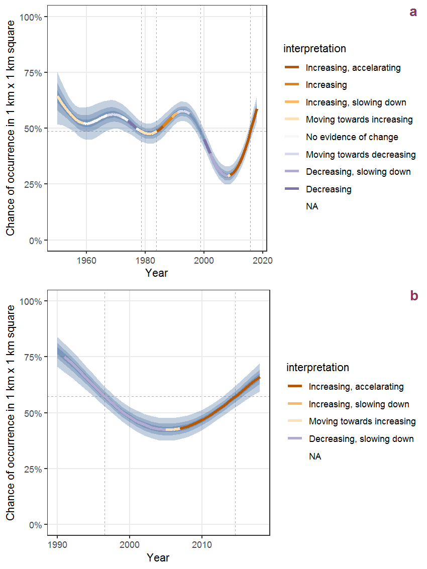
Figure B.37: Effect of year on the probability of Agrostis canina L. presence in 1 km x 1 km squares where the species has been observed at least once. The fitted line shows the sum of the overall mean (the intercept), a conditional effect of list-length equal to 130 and the year-smoother. The vertical dashed lines indicate the year(s) where the year-smoother is zero. The 95% confidence band is shown in grey (including the variability around the intercept and the smoother). a: 1950 - 2018, b: 1990 - 2018.
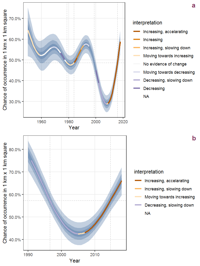
Figure B.38: The same as B.37, but the vertical axis is scaled to the range of the predicted values such that relative changes can be seen more easily. a: 1950 - 2018, b: 1990 - 2018.
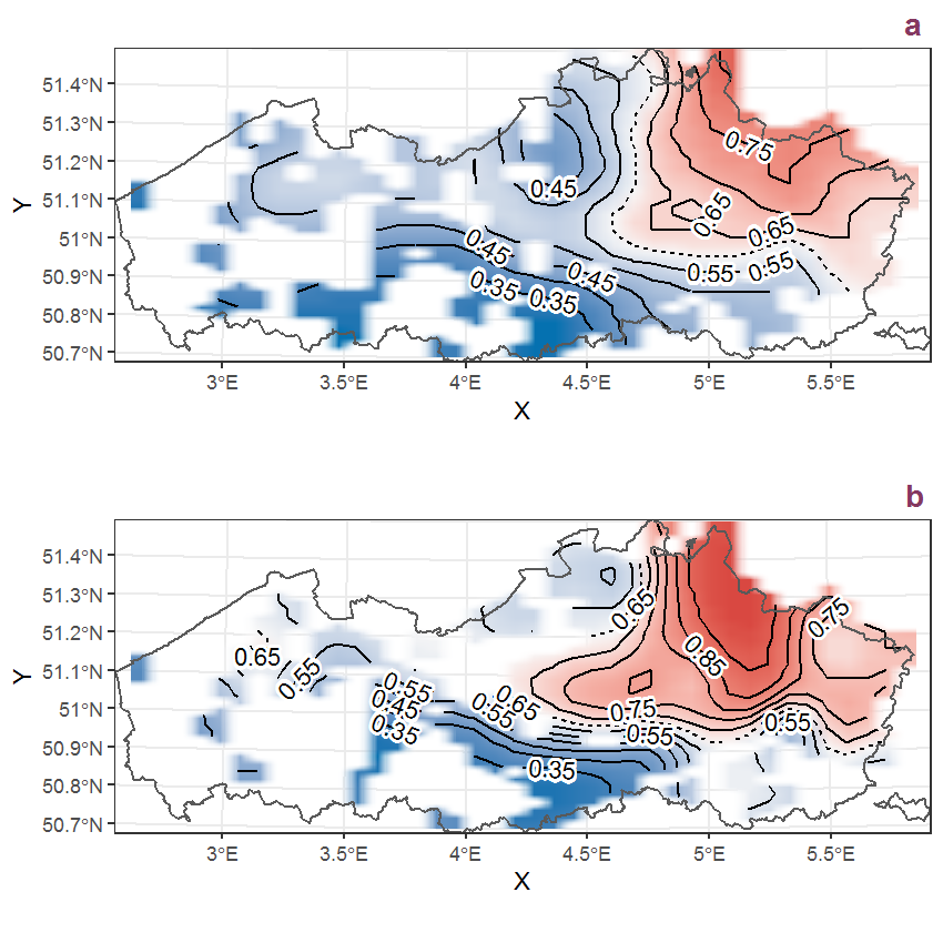
Figure B.39: Visualisation of the spatial smooth effect on the probability of Agrostis canina L. presence in 1 km x 1 km squares where the species has been observed at least once. The probabilities (values on the contour lines) are conditional on the final year of observation and a list-length equal to 130. The dashed contour line demarcates zones where the species is expected to be more prevalent (red shades) from zones where the species is less prevalent (blue shades). a: 1950 - 2018, b: 1990 - 2018.
B.14 Agrostis capillaris L.
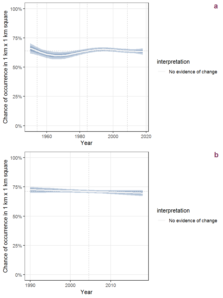
Figure B.40: Effect of year on the probability of Agrostis capillaris L. presence in 1 km x 1 km squares where the species has been observed at least once. The fitted line shows the sum of the overall mean (the intercept), a conditional effect of list-length equal to 130 and the year-smoother. The vertical dashed lines indicate the year(s) where the year-smoother is zero. The 95% confidence band is shown in grey (including the variability around the intercept and the smoother). a: 1950 - 2018, b: 1990 - 2018.
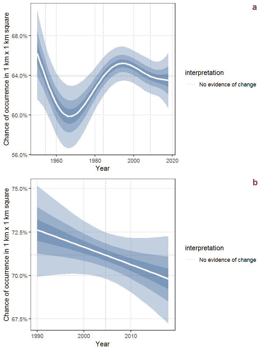
Figure B.41: The same as B.40, but the vertical axis is scaled to the range of the predicted values such that relative changes can be seen more easily. a: 1950 - 2018, b: 1990 - 2018.
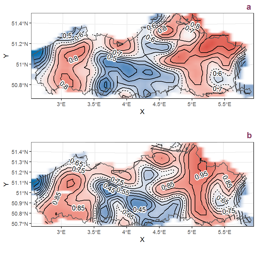
Figure B.42: Visualisation of the spatial smooth effect on the probability of Agrostis capillaris L. presence in 1 km x 1 km squares where the species has been observed at least once. The probabilities (values on the contour lines) are conditional on the final year of observation and a list-length equal to 130. The dashed contour line demarcates zones where the species is expected to be more prevalent (red shades) from zones where the species is less prevalent (blue shades). a: 1950 - 2018, b: 1990 - 2018.
B.15 Agrostis vinealis Schreb.
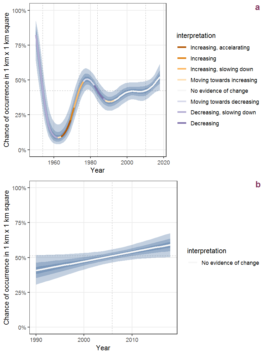
Figure B.43: Effect of year on the probability of Agrostis vinealis Schreb. presence in 1 km x 1 km squares where the species has been observed at least once. The fitted line shows the sum of the overall mean (the intercept), a conditional effect of list-length equal to 130 and the year-smoother. The vertical dashed lines indicate the year(s) where the year-smoother is zero. The 95% confidence band is shown in grey (including the variability around the intercept and the smoother). a: 1950 - 2018, b: 1990 - 2018.
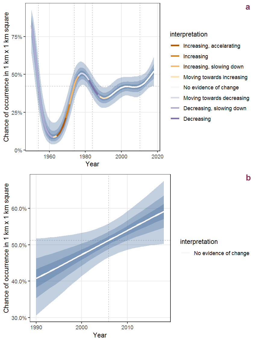
Figure B.44: The same as B.43, but the vertical axis is scaled to the range of the predicted values such that relative changes can be seen more easily. a: 1950 - 2018, b: 1990 - 2018.
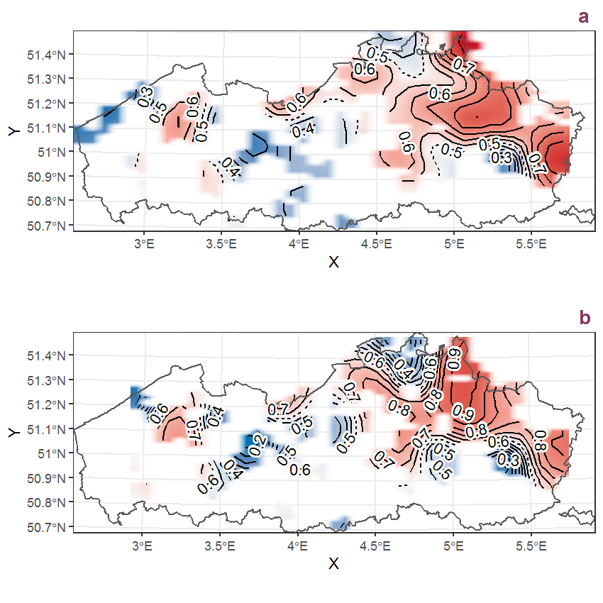
Figure B.45: Visualisation of the spatial smooth effect on the probability of Agrostis vinealis Schreb. presence in 1 km x 1 km squares where the species has been observed at least once. The probabilities (values on the contour lines) are conditional on the final year of observation and a list-length equal to 130. The dashed contour line demarcates zones where the species is expected to be more prevalent (red shades) from zones where the species is less prevalent (blue shades). a: 1950 - 2018, b: 1990 - 2018.
B.16 Ailanthus altissima (Mill.) Swingle
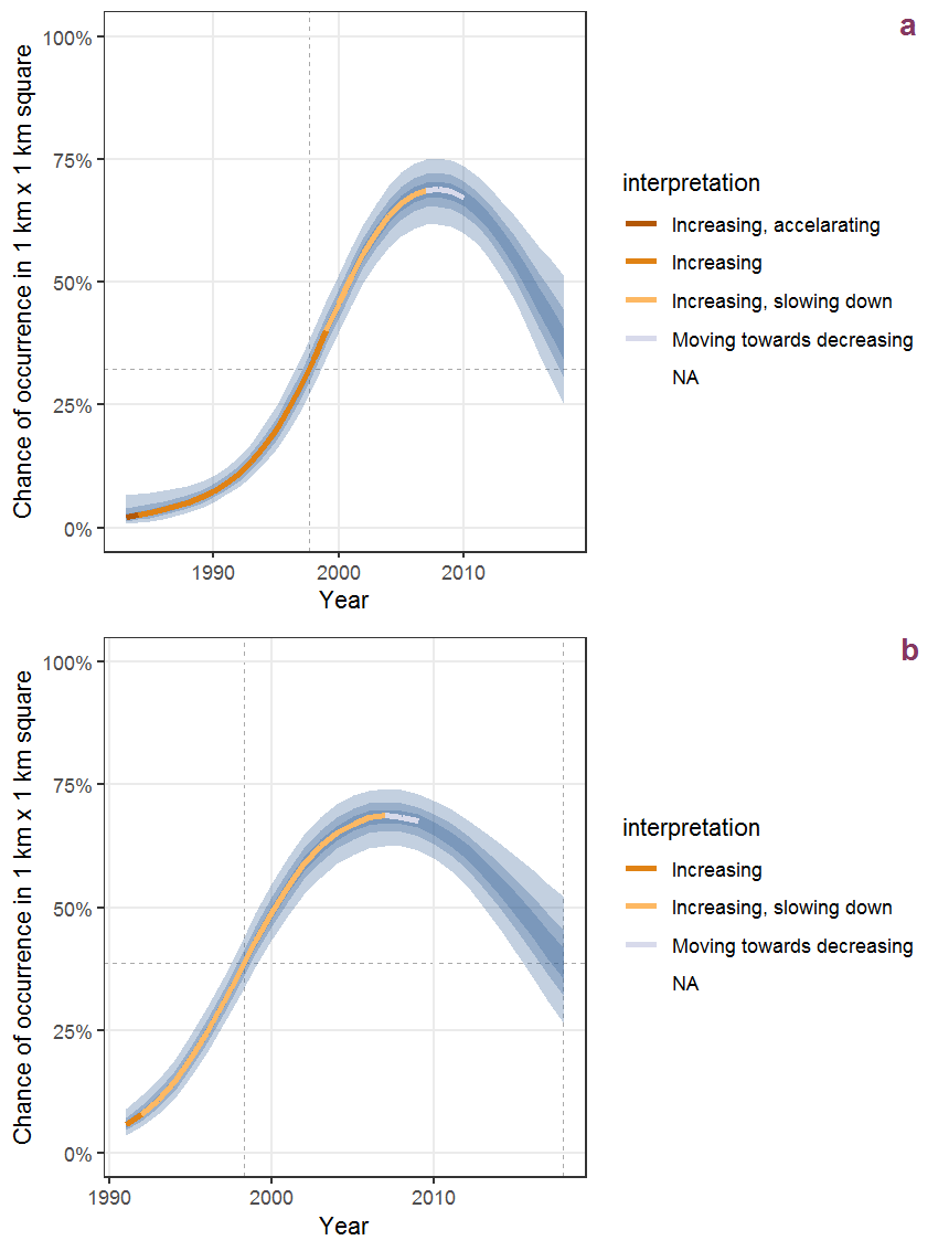
Figure B.46: Effect of year on the probability of Ailanthus altissima (Mill.) Swingle presence in 1 km x 1 km squares where the species has been observed at least once. The fitted line shows the sum of the overall mean (the intercept), a conditional effect of list-length equal to 130 and the year-smoother. The vertical dashed lines indicate the year(s) where the year-smoother is zero. The 95% confidence band is shown in grey (including the variability around the intercept and the smoother). a: 1950 - 2018, b: 1990 - 2018.
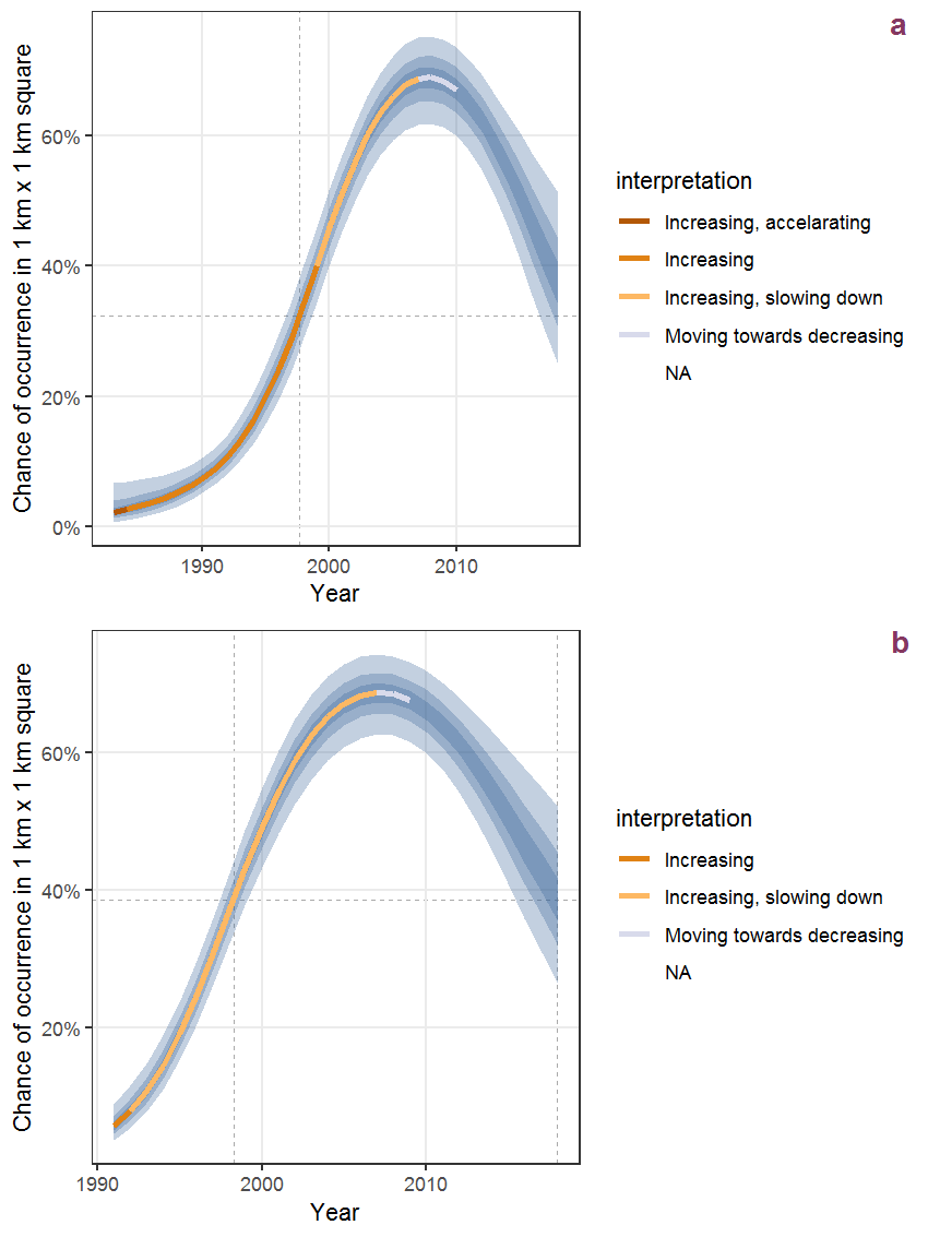
Figure B.47: The same as B.46, but the vertical axis is scaled to the range of the predicted values such that relative changes can be seen more easily. a: 1950 - 2018, b: 1990 - 2018.
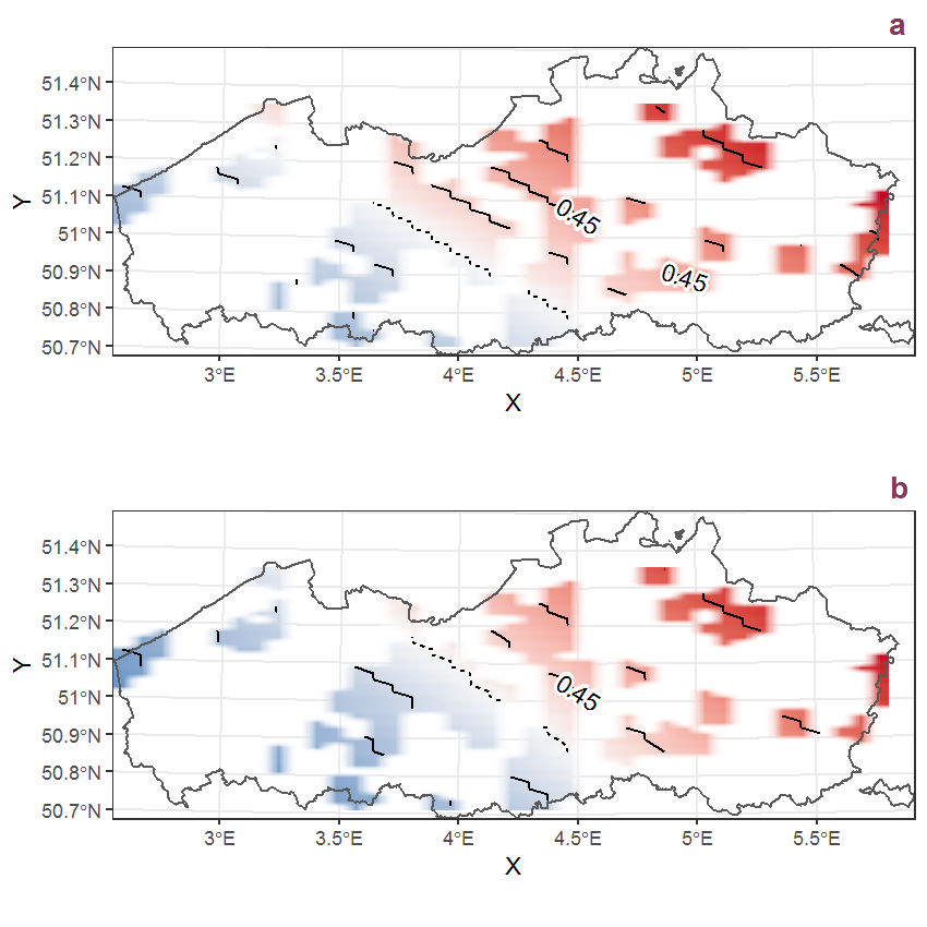
Figure B.48: Visualisation of the spatial smooth effect on the probability of Ailanthus altissima (Mill.) Swingle presence in 1 km x 1 km squares where the species has been observed at least once. The probabilities (values on the contour lines) are conditional on the final year of observation and a list-length equal to 130. The dashed contour line demarcates zones where the species is expected to be more prevalent (red shades) from zones where the species is less prevalent (blue shades). a: 1950 - 2018, b: 1990 - 2018.
B.17 Aira caryophyllea L.
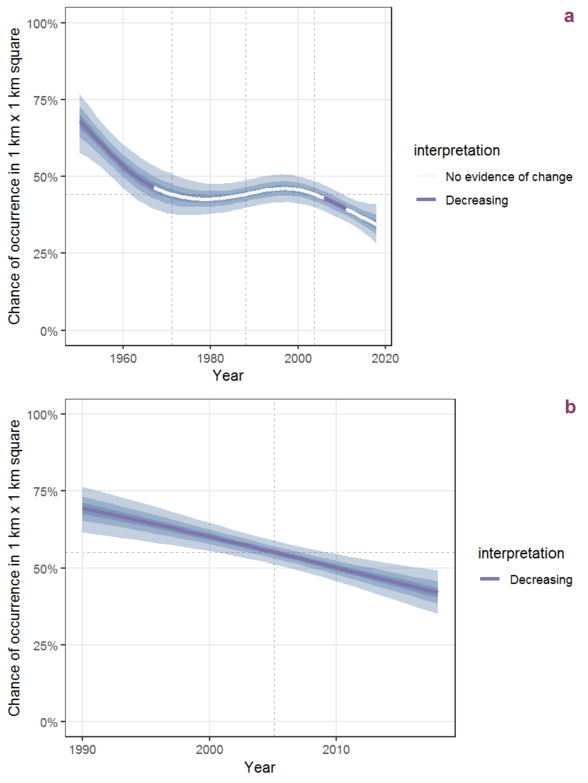
Figure B.49: Effect of year on the probability of Aira caryophyllea L. presence in 1 km x 1 km squares where the species has been observed at least once. The fitted line shows the sum of the overall mean (the intercept), a conditional effect of list-length equal to 130 and the year-smoother. The vertical dashed lines indicate the year(s) where the year-smoother is zero. The 95% confidence band is shown in grey (including the variability around the intercept and the smoother). a: 1950 - 2018, b: 1990 - 2018.
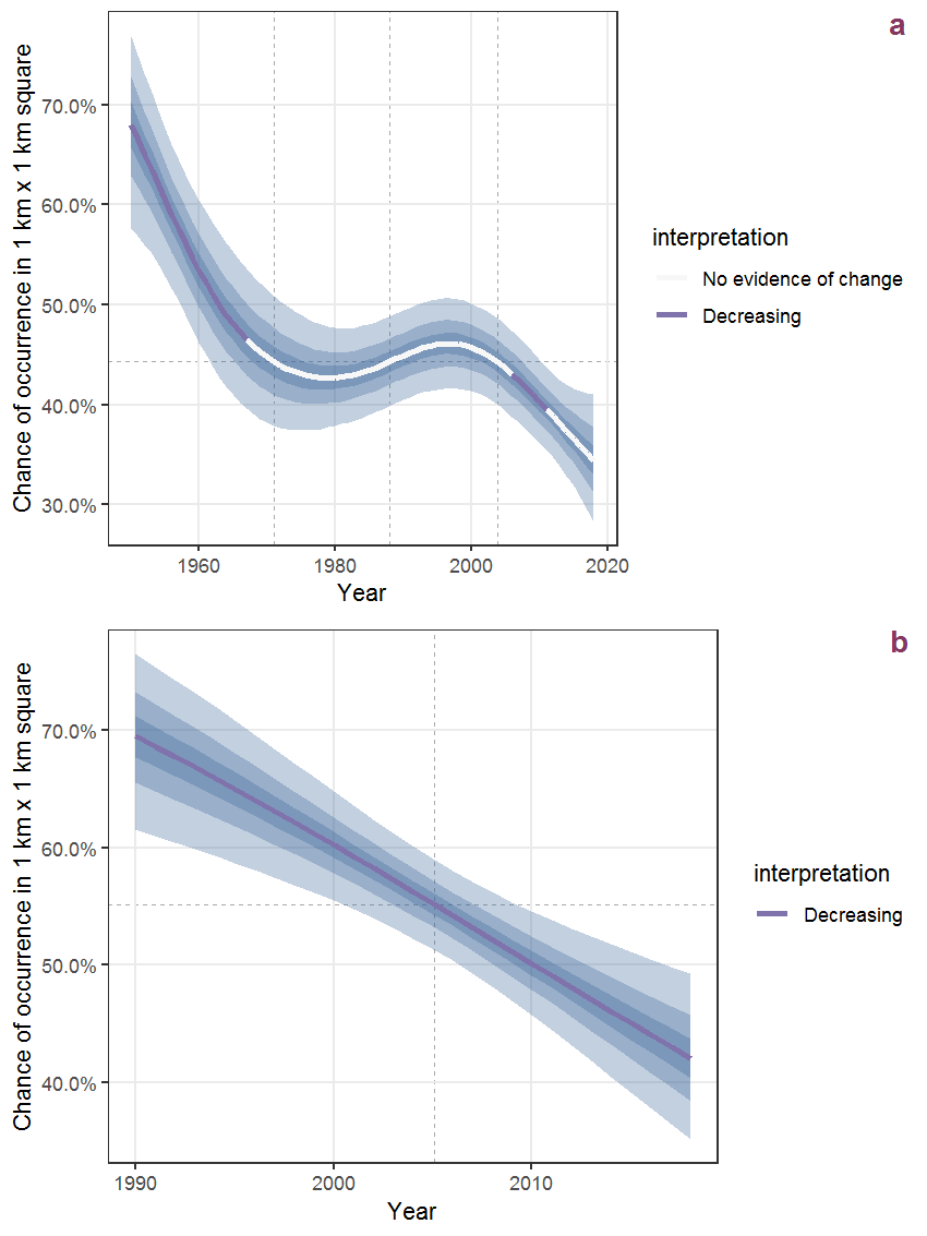
Figure B.50: The same as B.49, but the vertical axis is scaled to the range of the predicted values such that relative changes can be seen more easily. a: 1950 - 2018, b: 1990 - 2018.
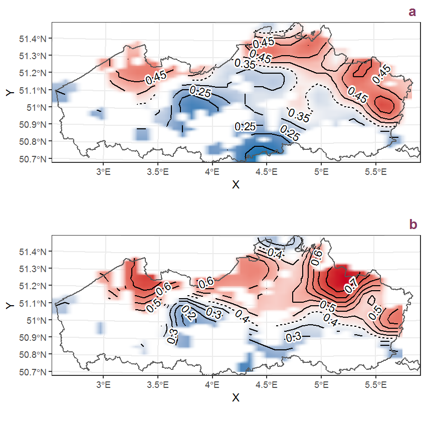
Figure B.51: Visualisation of the spatial smooth effect on the probability of Aira caryophyllea L. presence in 1 km x 1 km squares where the species has been observed at least once. The probabilities (values on the contour lines) are conditional on the final year of observation and a list-length equal to 130. The dashed contour line demarcates zones where the species is expected to be more prevalent (red shades) from zones where the species is less prevalent (blue shades). a: 1950 - 2018, b: 1990 - 2018.
B.18 Aira praecox L.
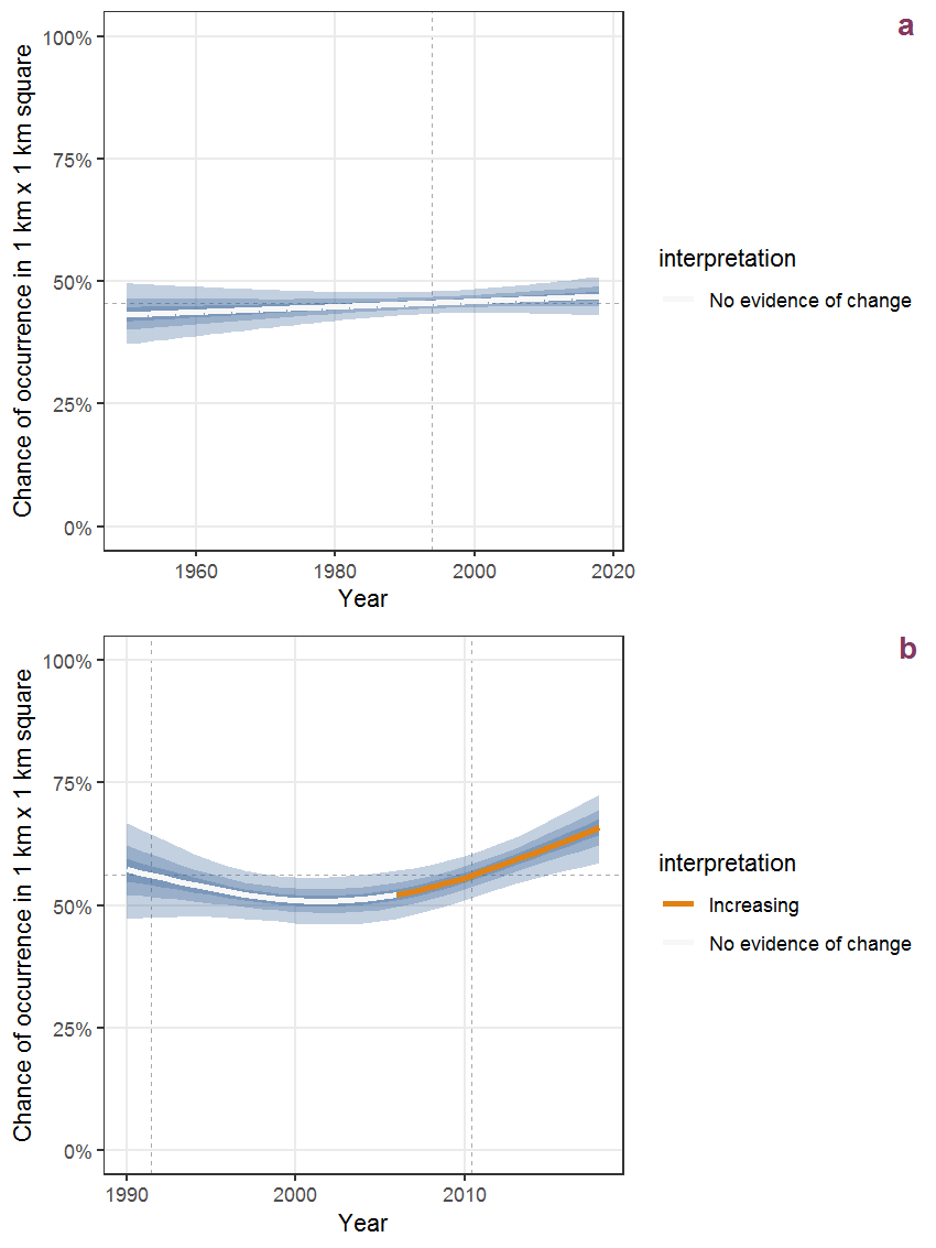
Figure B.52: Effect of year on the probability of Aira praecox L. presence in 1 km x 1 km squares where the species has been observed at least once. The fitted line shows the sum of the overall mean (the intercept), a conditional effect of list-length equal to 130 and the year-smoother. The vertical dashed lines indicate the year(s) where the year-smoother is zero. The 95% confidence band is shown in grey (including the variability around the intercept and the smoother). a: 1950 - 2018, b: 1990 - 2018.
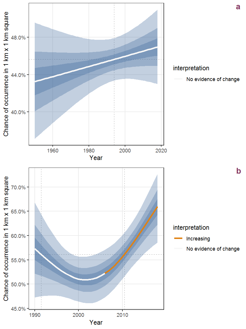
Figure B.53: The same as B.52, but the vertical axis is scaled to the range of the predicted values such that relative changes can be seen more easily. a: 1950 - 2018, b: 1990 - 2018.
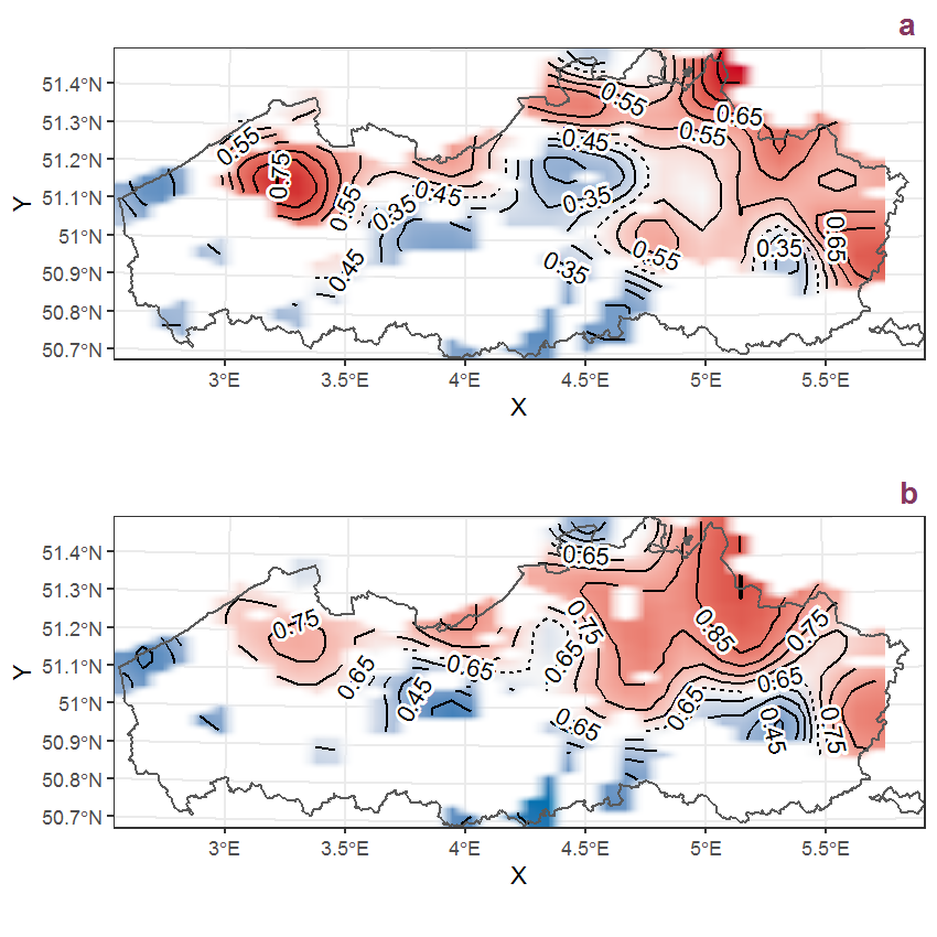
Figure B.54: Visualisation of the spatial smooth effect on the probability of Aira praecox L. presence in 1 km x 1 km squares where the species has been observed at least once. The probabilities (values on the contour lines) are conditional on the final year of observation and a list-length equal to 130. The dashed contour line demarcates zones where the species is expected to be more prevalent (red shades) from zones where the species is less prevalent (blue shades). a: 1950 - 2018, b: 1990 - 2018.
B.19 Ajuga reptans L.
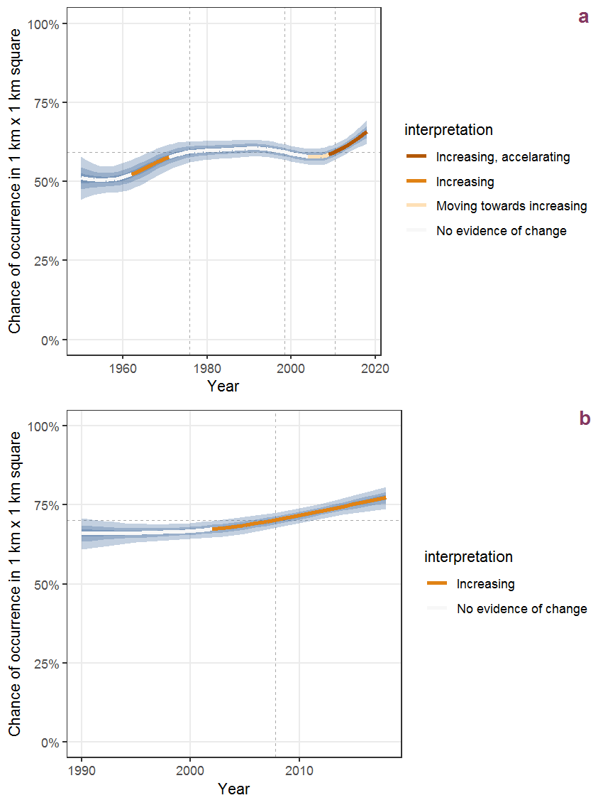
Figure B.55: Effect of year on the probability of Ajuga reptans L. presence in 1 km x 1 km squares where the species has been observed at least once. The fitted line shows the sum of the overall mean (the intercept), a conditional effect of list-length equal to 130 and the year-smoother. The vertical dashed lines indicate the year(s) where the year-smoother is zero. The 95% confidence band is shown in grey (including the variability around the intercept and the smoother). a: 1950 - 2018, b: 1990 - 2018.
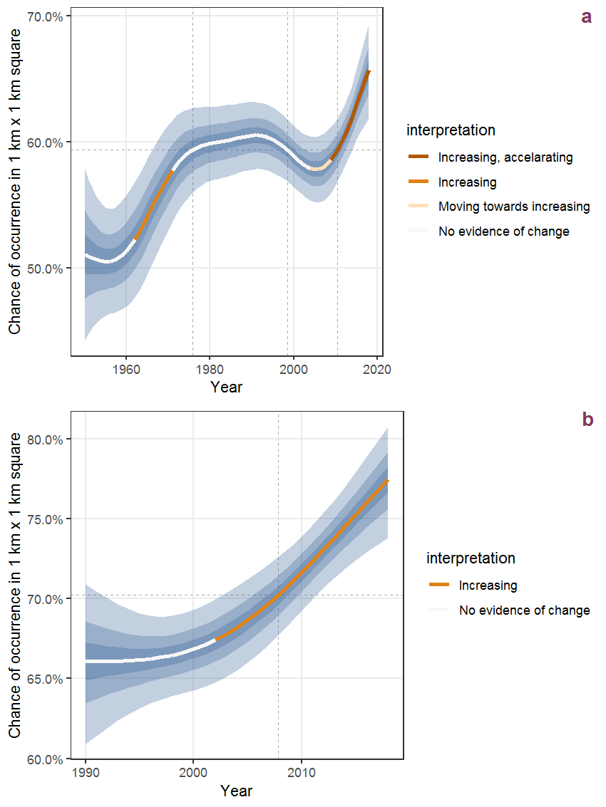
Figure B.56: The same as B.55, but the vertical axis is scaled to the range of the predicted values such that relative changes can be seen more easily. a: 1950 - 2018, b: 1990 - 2018.
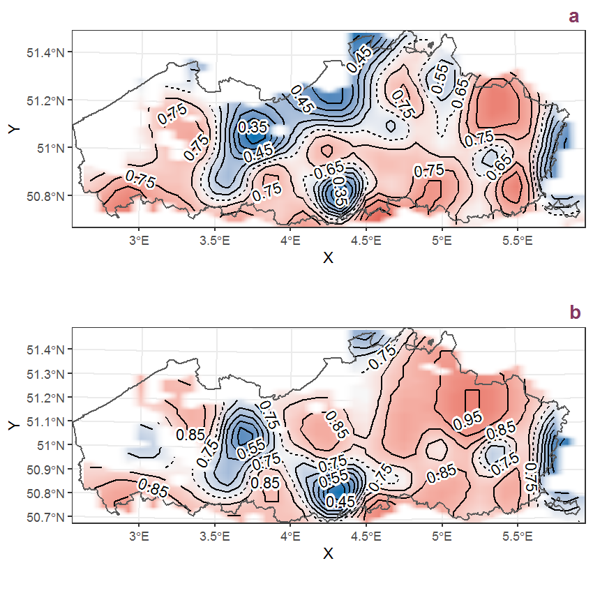
Figure B.57: Visualisation of the spatial smooth effect on the probability of Ajuga reptans L. presence in 1 km x 1 km squares where the species has been observed at least once. The probabilities (values on the contour lines) are conditional on the final year of observation and a list-length equal to 130. The dashed contour line demarcates zones where the species is expected to be more prevalent (red shades) from zones where the species is less prevalent (blue shades). a: 1950 - 2018, b: 1990 - 2018.
B.20 Alchemilla mollis (Buser) Rothm.
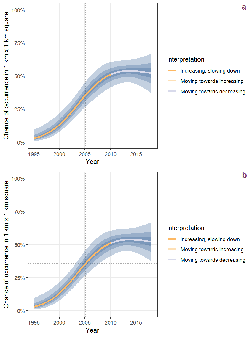
Figure B.58: Effect of year on the probability of Alchemilla mollis (Buser) Rothm. presence in 1 km x 1 km squares where the species has been observed at least once. The fitted line shows the sum of the overall mean (the intercept), a conditional effect of list-length equal to 130 and the year-smoother. The vertical dashed lines indicate the year(s) where the year-smoother is zero. The 95% confidence band is shown in grey (including the variability around the intercept and the smoother). a: 1950 - 2018, b: 1990 - 2018.
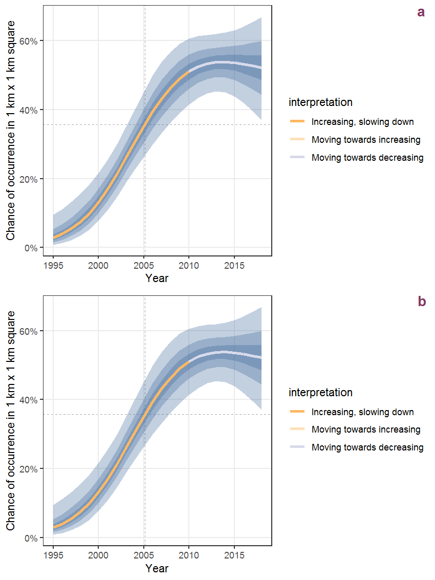
Figure B.59: The same as B.58, but the vertical axis is scaled to the range of the predicted values such that relative changes can be seen more easily. a: 1950 - 2018, b: 1990 - 2018.
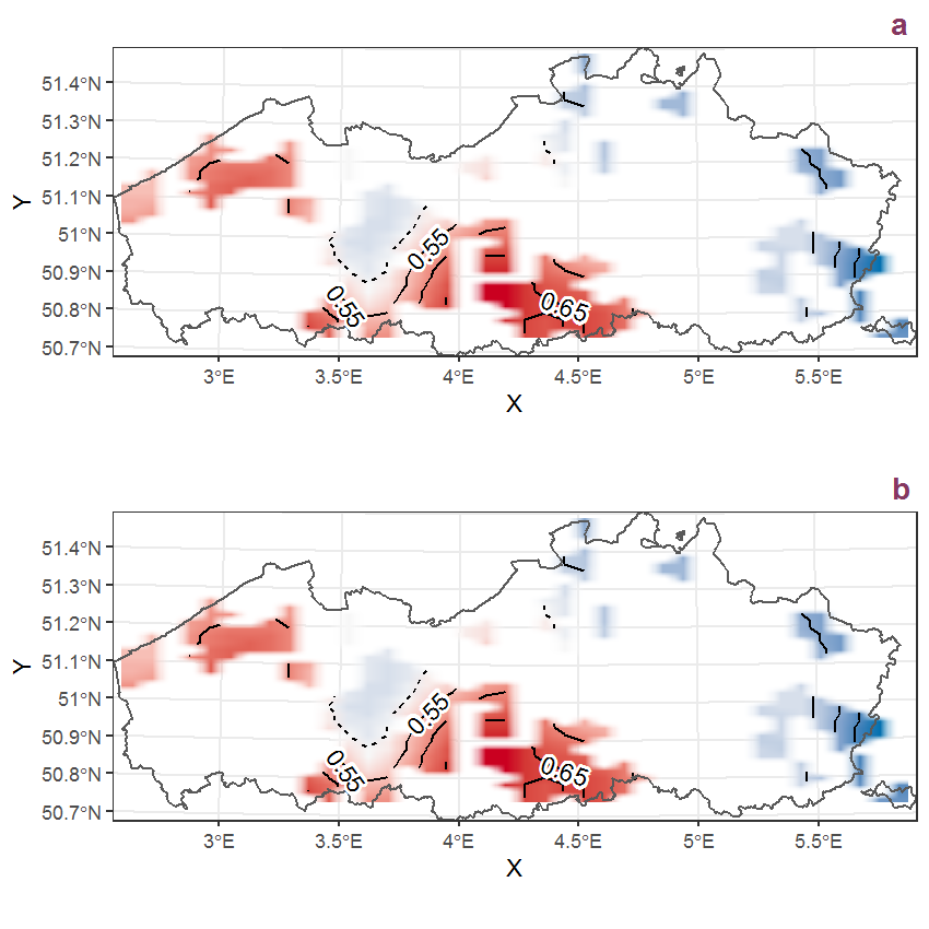
Figure B.60: Visualisation of the spatial smooth effect on the probability of Alchemilla mollis (Buser) Rothm. presence in 1 km x 1 km squares where the species has been observed at least once. The probabilities (values on the contour lines) are conditional on the final year of observation and a list-length equal to 130. The dashed contour line demarcates zones where the species is expected to be more prevalent (red shades) from zones where the species is less prevalent (blue shades). a: 1950 - 2018, b: 1990 - 2018.
B.21 Alisma plantago-aquatica L.
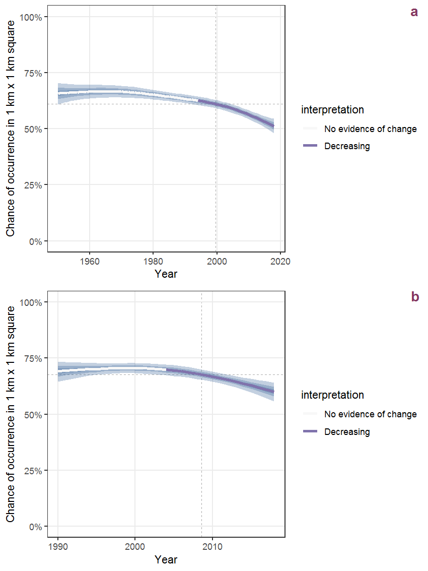
Figure B.61: Effect of year on the probability of Alisma plantago-aquatica L. presence in 1 km x 1 km squares where the species has been observed at least once. The fitted line shows the sum of the overall mean (the intercept), a conditional effect of list-length equal to 130 and the year-smoother. The vertical dashed lines indicate the year(s) where the year-smoother is zero. The 95% confidence band is shown in grey (including the variability around the intercept and the smoother). a: 1950 - 2018, b: 1990 - 2018.
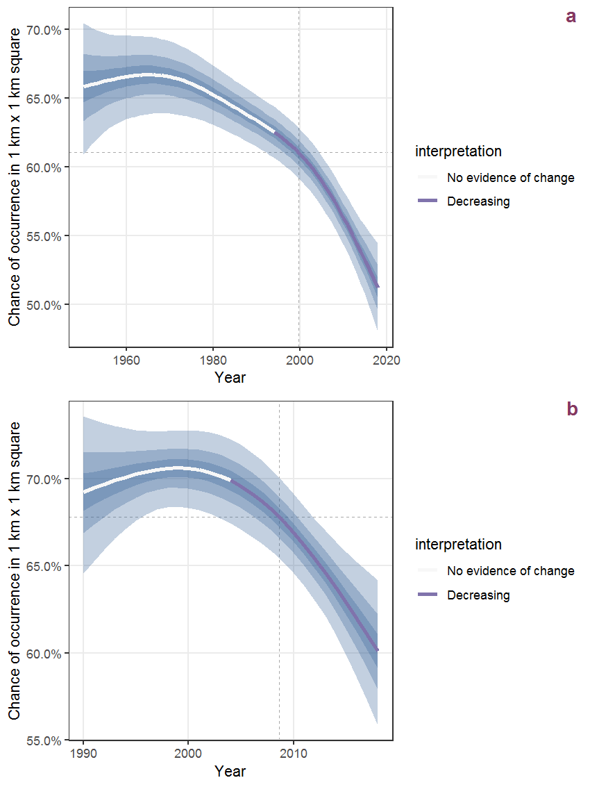
Figure B.62: The same as B.61, but the vertical axis is scaled to the range of the predicted values such that relative changes can be seen more easily. a: 1950 - 2018, b: 1990 - 2018.
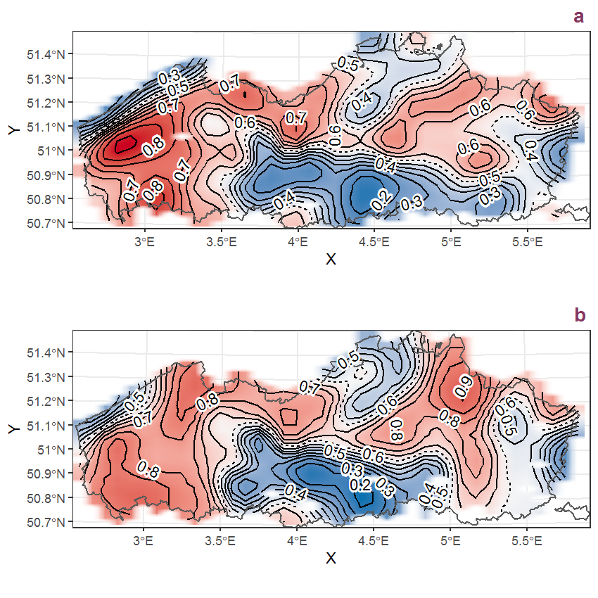
Figure B.63: Visualisation of the spatial smooth effect on the probability of Alisma plantago-aquatica L. presence in 1 km x 1 km squares where the species has been observed at least once. The probabilities (values on the contour lines) are conditional on the final year of observation and a list-length equal to 130. The dashed contour line demarcates zones where the species is expected to be more prevalent (red shades) from zones where the species is less prevalent (blue shades). a: 1950 - 2018, b: 1990 - 2018.
B.22 Alliaria petiolata (Bieb.) Cavara et Grande
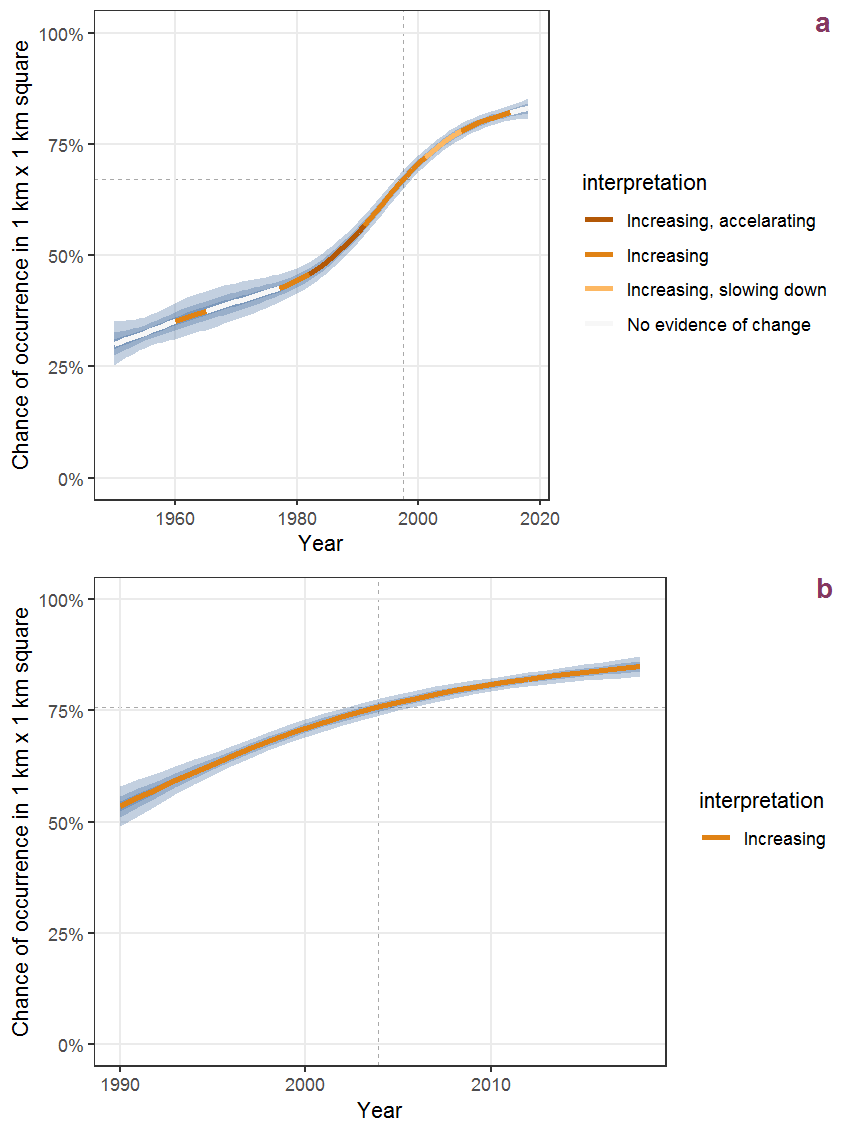
Figure B.64: Effect of year on the probability of Alliaria petiolata (Bieb.) Cavara et Grande presence in 1 km x 1 km squares where the species has been observed at least once. The fitted line shows the sum of the overall mean (the intercept), a conditional effect of list-length equal to 130 and the year-smoother. The vertical dashed lines indicate the year(s) where the year-smoother is zero. The 95% confidence band is shown in grey (including the variability around the intercept and the smoother). a: 1950 - 2018, b: 1990 - 2018.
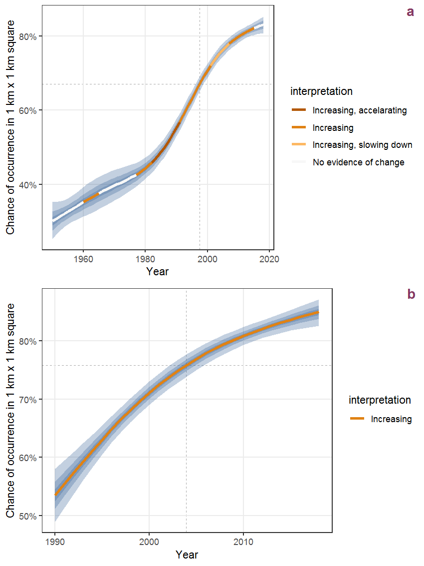
Figure B.65: The same as B.64, but the vertical axis is scaled to the range of the predicted values such that relative changes can be seen more easily. a: 1950 - 2018, b: 1990 - 2018.
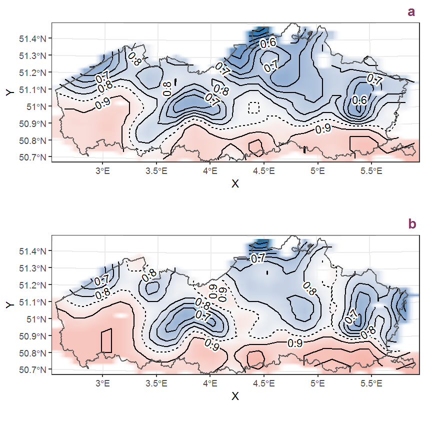
Figure B.66: Visualisation of the spatial smooth effect on the probability of Alliaria petiolata (Bieb.) Cavara et Grande presence in 1 km x 1 km squares where the species has been observed at least once. The probabilities (values on the contour lines) are conditional on the final year of observation and a list-length equal to 130. The dashed contour line demarcates zones where the species is expected to be more prevalent (red shades) from zones where the species is less prevalent (blue shades). a: 1950 - 2018, b: 1990 - 2018.
B.23 Allium ursinum L.
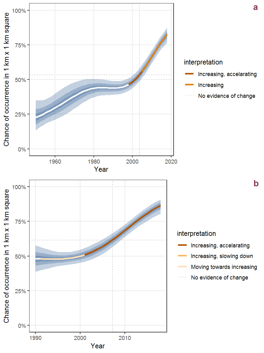
Figure B.67: Effect of year on the probability of Allium ursinum L. presence in 1 km x 1 km squares where the species has been observed at least once. The fitted line shows the sum of the overall mean (the intercept), a conditional effect of list-length equal to 130 and the year-smoother. The vertical dashed lines indicate the year(s) where the year-smoother is zero. The 95% confidence band is shown in grey (including the variability around the intercept and the smoother). a: 1950 - 2018, b: 1990 - 2018.
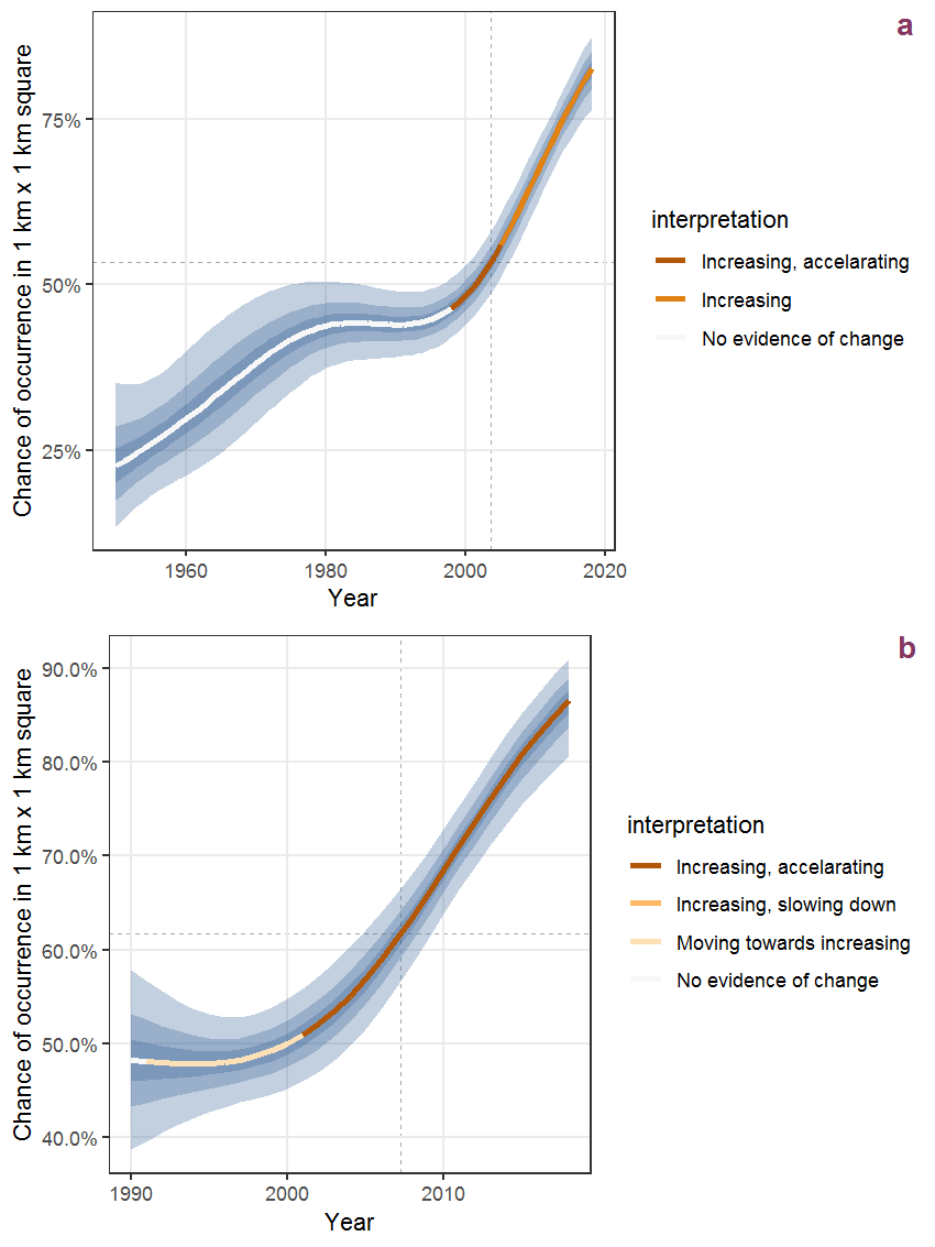
Figure B.68: The same as B.67, but the vertical axis is scaled to the range of the predicted values such that relative changes can be seen more easily. a: 1950 - 2018, b: 1990 - 2018.
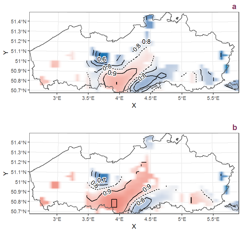
Figure B.69: Visualisation of the spatial smooth effect on the probability of Allium ursinum L. presence in 1 km x 1 km squares where the species has been observed at least once. The probabilities (values on the contour lines) are conditional on the final year of observation and a list-length equal to 130. The dashed contour line demarcates zones where the species is expected to be more prevalent (red shades) from zones where the species is less prevalent (blue shades). a: 1950 - 2018, b: 1990 - 2018.
B.24 Allium vineale L.
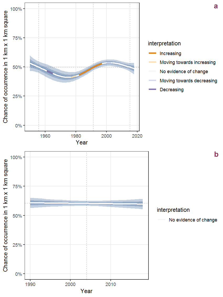
Figure B.70: Effect of year on the probability of Allium vineale L. presence in 1 km x 1 km squares where the species has been observed at least once. The fitted line shows the sum of the overall mean (the intercept), a conditional effect of list-length equal to 130 and the year-smoother. The vertical dashed lines indicate the year(s) where the year-smoother is zero. The 95% confidence band is shown in grey (including the variability around the intercept and the smoother). a: 1950 - 2018, b: 1990 - 2018.
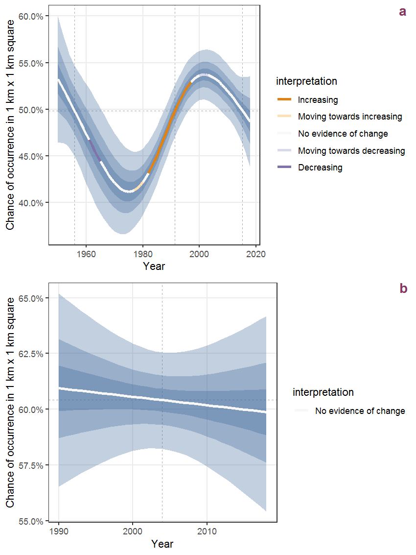
Figure B.71: The same as B.70, but the vertical axis is scaled to the range of the predicted values such that relative changes can be seen more easily. a: 1950 - 2018, b: 1990 - 2018.
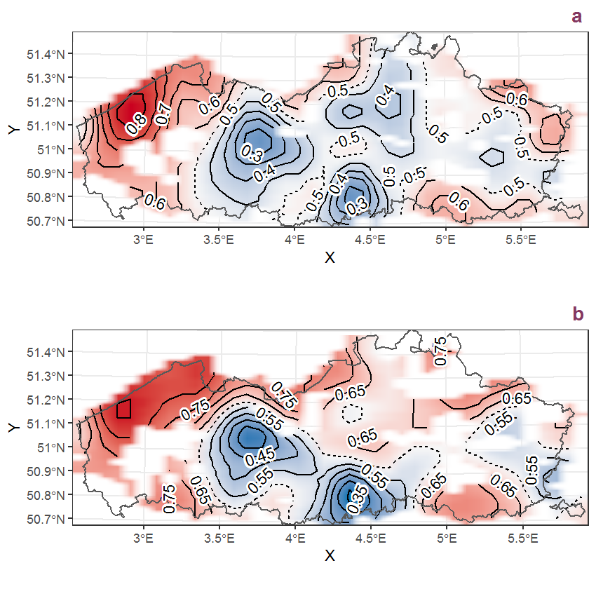
Figure B.72: Visualisation of the spatial smooth effect on the probability of Allium vineale L. presence in 1 km x 1 km squares where the species has been observed at least once. The probabilities (values on the contour lines) are conditional on the final year of observation and a list-length equal to 130. The dashed contour line demarcates zones where the species is expected to be more prevalent (red shades) from zones where the species is less prevalent (blue shades). a: 1950 - 2018, b: 1990 - 2018.
B.25 Alnus glutinosa (L.) Gaertn.
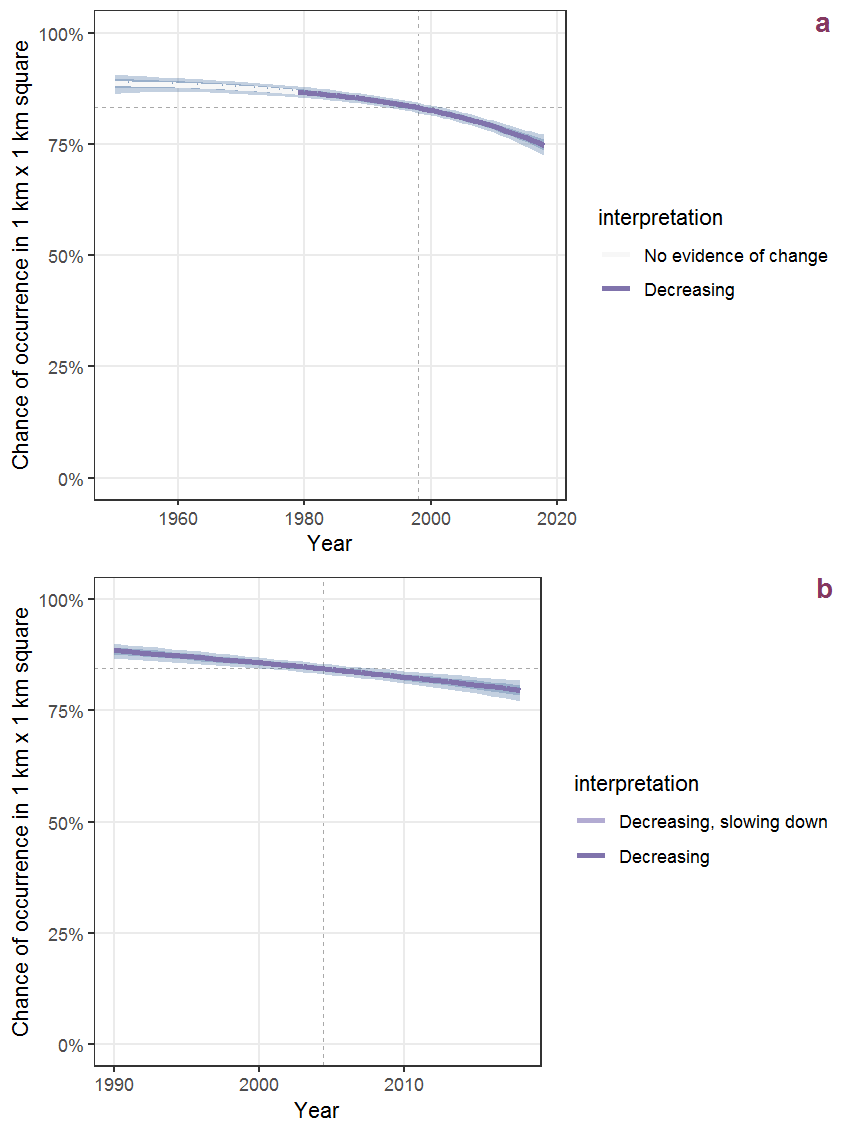
Figure B.73: Effect of year on the probability of Alnus glutinosa (L.) Gaertn. presence in 1 km x 1 km squares where the species has been observed at least once. The fitted line shows the sum of the overall mean (the intercept), a conditional effect of list-length equal to 130 and the year-smoother. The vertical dashed lines indicate the year(s) where the year-smoother is zero. The 95% confidence band is shown in grey (including the variability around the intercept and the smoother). a: 1950 - 2018, b: 1990 - 2018.
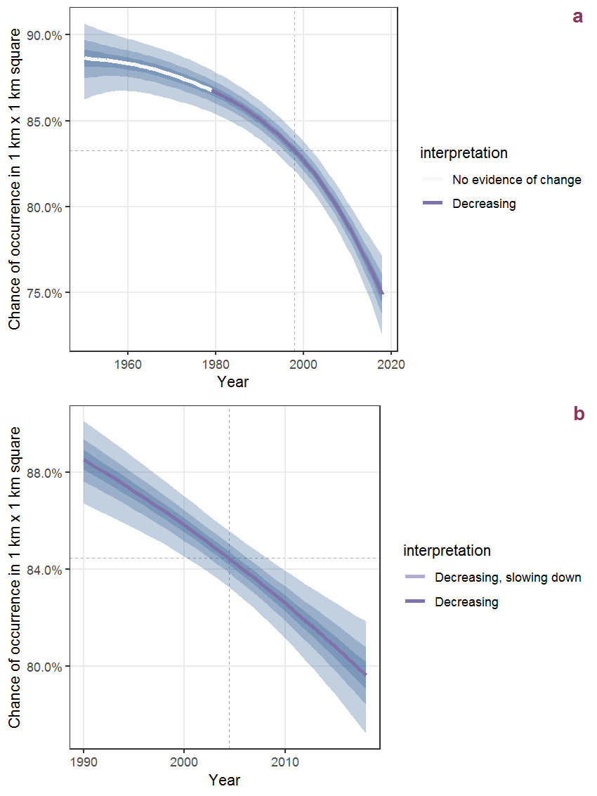
Figure B.74: The same as B.73, but the vertical axis is scaled to the range of the predicted values such that relative changes can be seen more easily. a: 1950 - 2018, b: 1990 - 2018.
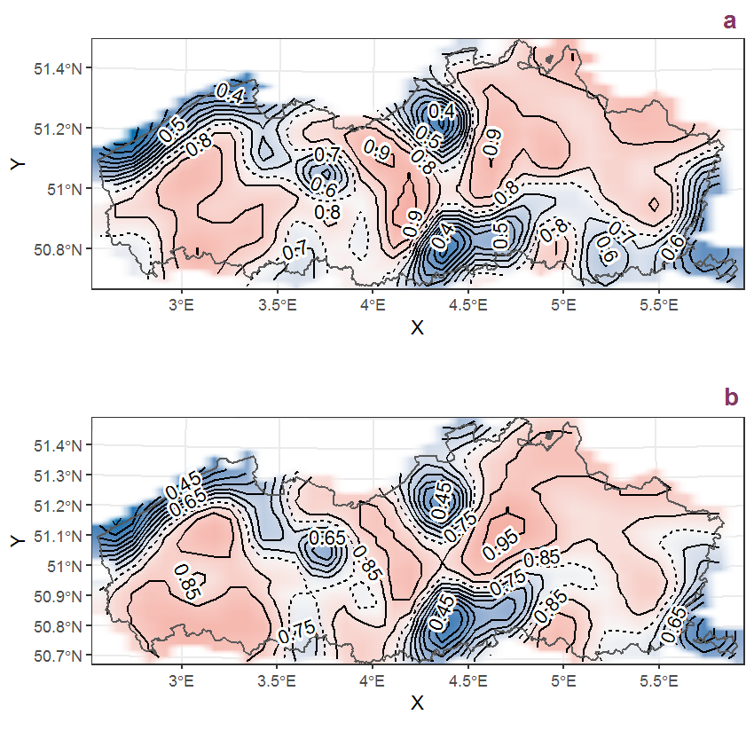
Figure B.75: Visualisation of the spatial smooth effect on the probability of Alnus glutinosa (L.) Gaertn. presence in 1 km x 1 km squares where the species has been observed at least once. The probabilities (values on the contour lines) are conditional on the final year of observation and a list-length equal to 130. The dashed contour line demarcates zones where the species is expected to be more prevalent (red shades) from zones where the species is less prevalent (blue shades). a: 1950 - 2018, b: 1990 - 2018.
B.26 Alnus incana (L.) Moench
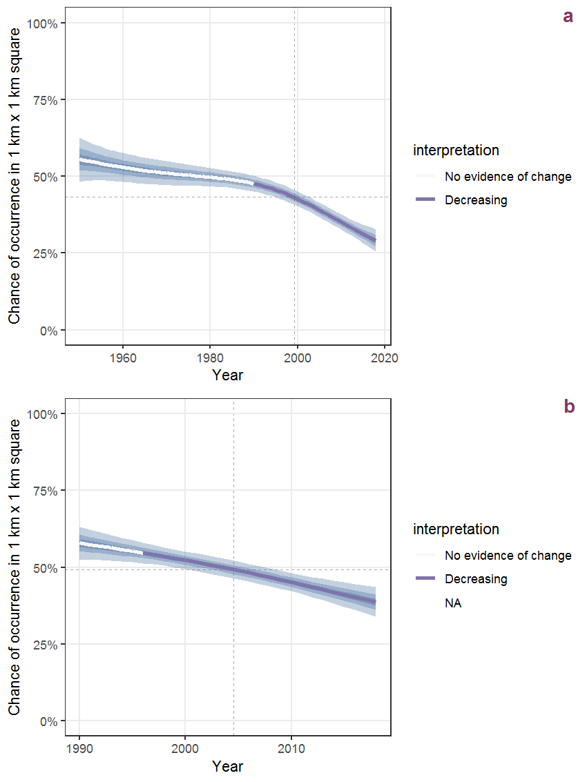
Figure B.76: Effect of year on the probability of Alnus incana (L.) Moench presence in 1 km x 1 km squares where the species has been observed at least once. The fitted line shows the sum of the overall mean (the intercept), a conditional effect of list-length equal to 130 and the year-smoother. The vertical dashed lines indicate the year(s) where the year-smoother is zero. The 95% confidence band is shown in grey (including the variability around the intercept and the smoother). a: 1950 - 2018, b: 1990 - 2018.
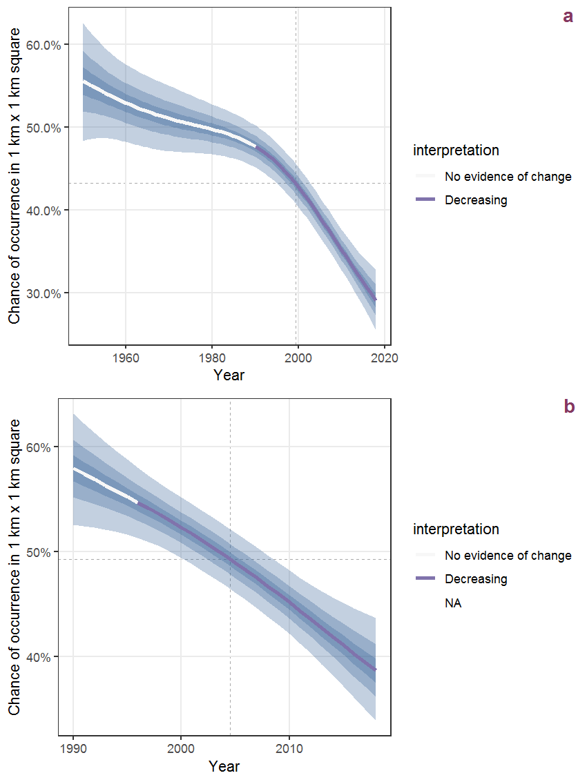
Figure B.77: The same as B.76, but the vertical axis is scaled to the range of the predicted values such that relative changes can be seen more easily. a: 1950 - 2018, b: 1990 - 2018.
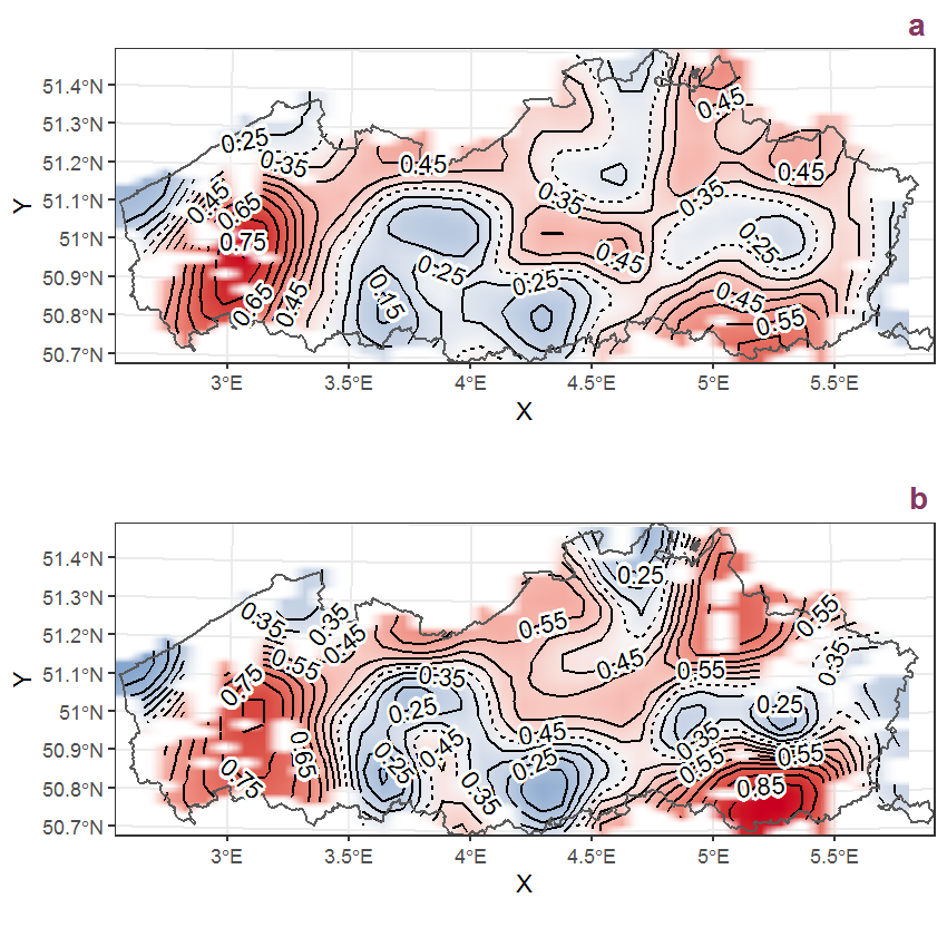
Figure B.78: Visualisation of the spatial smooth effect on the probability of Alnus incana (L.) Moench presence in 1 km x 1 km squares where the species has been observed at least once. The probabilities (values on the contour lines) are conditional on the final year of observation and a list-length equal to 130. The dashed contour line demarcates zones where the species is expected to be more prevalent (red shades) from zones where the species is less prevalent (blue shades). a: 1950 - 2018, b: 1990 - 2018.
B.27 Alopecurus geniculatus L.
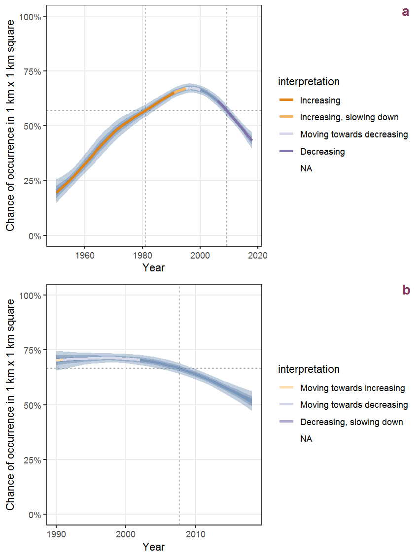
Figure B.79: Effect of year on the probability of Alopecurus geniculatus L. presence in 1 km x 1 km squares where the species has been observed at least once. The fitted line shows the sum of the overall mean (the intercept), a conditional effect of list-length equal to 130 and the year-smoother. The vertical dashed lines indicate the year(s) where the year-smoother is zero. The 95% confidence band is shown in grey (including the variability around the intercept and the smoother). a: 1950 - 2018, b: 1990 - 2018.
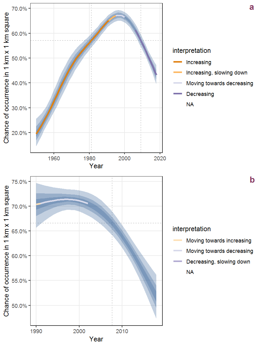
Figure B.80: The same as B.79, but the vertical axis is scaled to the range of the predicted values such that relative changes can be seen more easily. a: 1950 - 2018, b: 1990 - 2018.
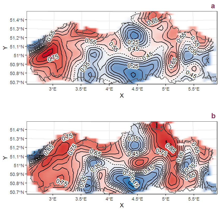
Figure B.81: Visualisation of the spatial smooth effect on the probability of Alopecurus geniculatus L. presence in 1 km x 1 km squares where the species has been observed at least once. The probabilities (values on the contour lines) are conditional on the final year of observation and a list-length equal to 130. The dashed contour line demarcates zones where the species is expected to be more prevalent (red shades) from zones where the species is less prevalent (blue shades). a: 1950 - 2018, b: 1990 - 2018.
B.28 Alopecurus myosuroides Huds.
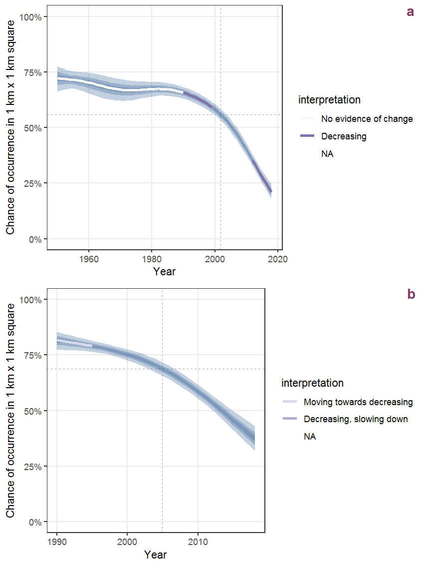
Figure B.82: Effect of year on the probability of Alopecurus myosuroides Huds. presence in 1 km x 1 km squares where the species has been observed at least once. The fitted line shows the sum of the overall mean (the intercept), a conditional effect of list-length equal to 130 and the year-smoother. The vertical dashed lines indicate the year(s) where the year-smoother is zero. The 95% confidence band is shown in grey (including the variability around the intercept and the smoother). a: 1950 - 2018, b: 1990 - 2018.
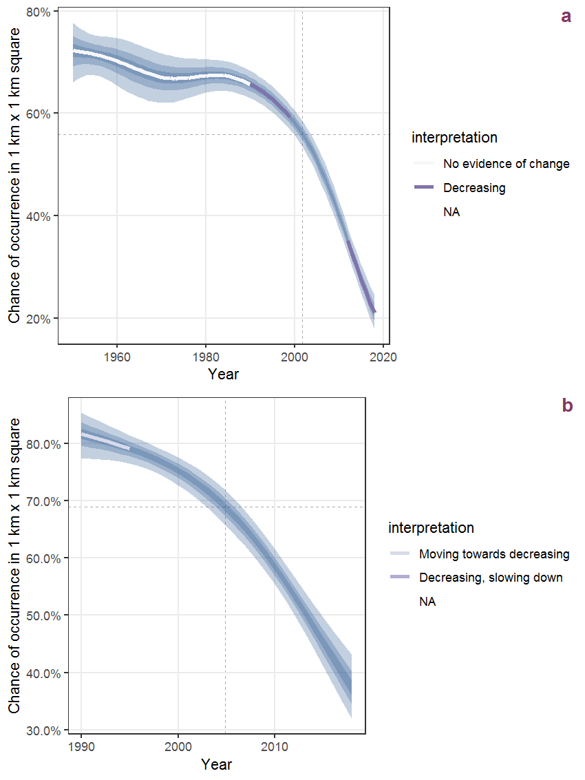
Figure B.83: The same as B.82, but the vertical axis is scaled to the range of the predicted values such that relative changes can be seen more easily. a: 1950 - 2018, b: 1990 - 2018.
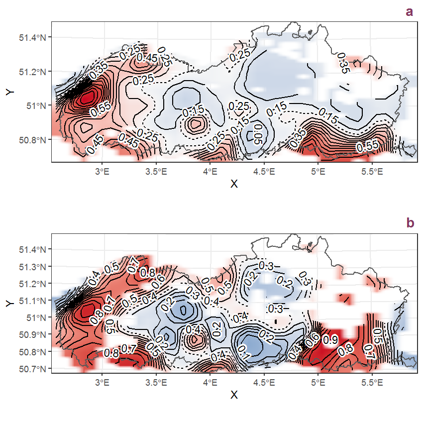
Figure B.84: Visualisation of the spatial smooth effect on the probability of Alopecurus myosuroides Huds. presence in 1 km x 1 km squares where the species has been observed at least once. The probabilities (values on the contour lines) are conditional on the final year of observation and a list-length equal to 130. The dashed contour line demarcates zones where the species is expected to be more prevalent (red shades) from zones where the species is less prevalent (blue shades). a: 1950 - 2018, b: 1990 - 2018.
B.29 Alopecurus pratensis L.
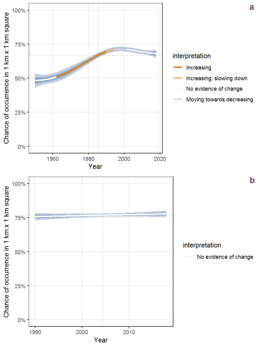
Figure B.85: Effect of year on the probability of Alopecurus pratensis L. presence in 1 km x 1 km squares where the species has been observed at least once. The fitted line shows the sum of the overall mean (the intercept), a conditional effect of list-length equal to 130 and the year-smoother. The vertical dashed lines indicate the year(s) where the year-smoother is zero. The 95% confidence band is shown in grey (including the variability around the intercept and the smoother). a: 1950 - 2018, b: 1990 - 2018.
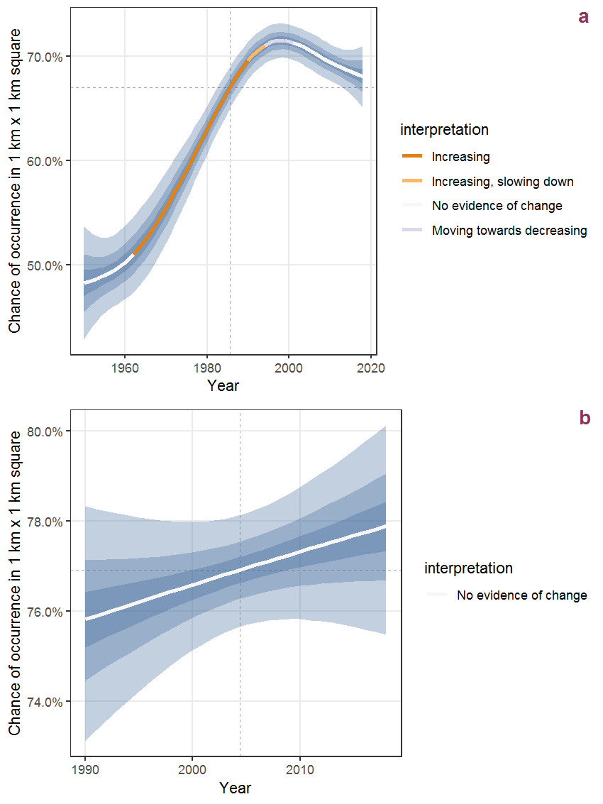
Figure B.86: The same as B.85, but the vertical axis is scaled to the range of the predicted values such that relative changes can be seen more easily. a: 1950 - 2018, b: 1990 - 2018.
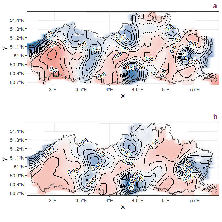
Figure B.87: Visualisation of the spatial smooth effect on the probability of Alopecurus pratensis L. presence in 1 km x 1 km squares where the species has been observed at least once. The probabilities (values on the contour lines) are conditional on the final year of observation and a list-length equal to 130. The dashed contour line demarcates zones where the species is expected to be more prevalent (red shades) from zones where the species is less prevalent (blue shades). a: 1950 - 2018, b: 1990 - 2018.
B.30 Amaranthus blitum L.
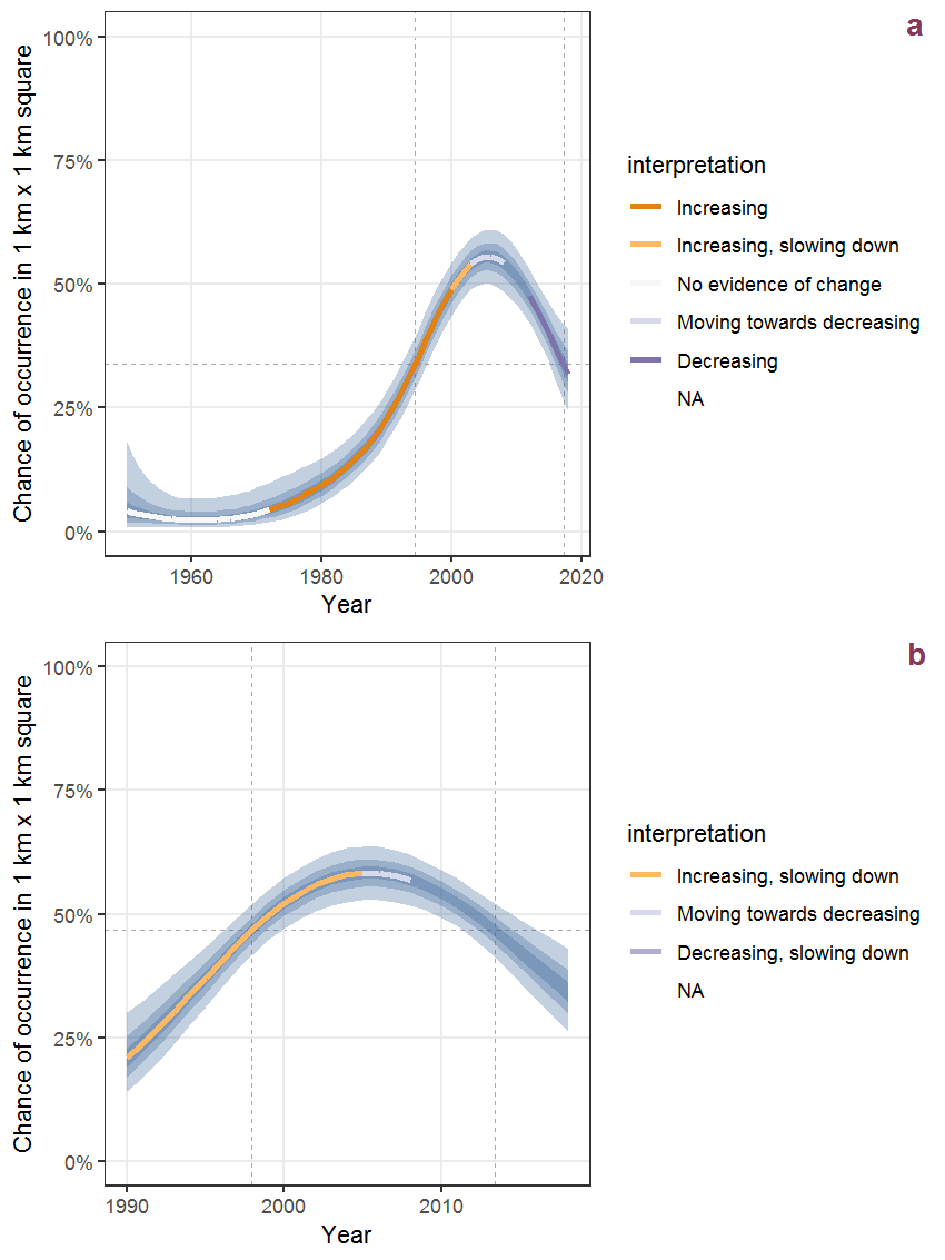
Figure B.88: Effect of year on the probability of Amaranthus blitum L. presence in 1 km x 1 km squares where the species has been observed at least once. The fitted line shows the sum of the overall mean (the intercept), a conditional effect of list-length equal to 130 and the year-smoother. The vertical dashed lines indicate the year(s) where the year-smoother is zero. The 95% confidence band is shown in grey (including the variability around the intercept and the smoother). a: 1950 - 2018, b: 1990 - 2018.
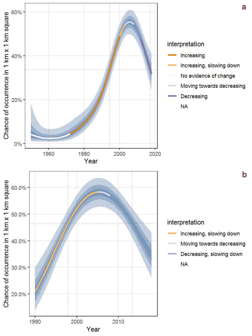
Figure B.89: The same as B.88, but the vertical axis is scaled to the range of the predicted values such that relative changes can be seen more easily. a: 1950 - 2018, b: 1990 - 2018.
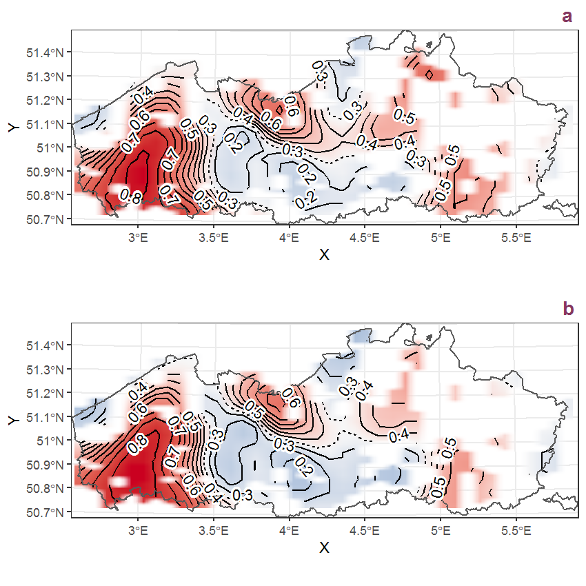
Figure B.90: Visualisation of the spatial smooth effect on the probability of Amaranthus blitum L. presence in 1 km x 1 km squares where the species has been observed at least once. The probabilities (values on the contour lines) are conditional on the final year of observation and a list-length equal to 130. The dashed contour line demarcates zones where the species is expected to be more prevalent (red shades) from zones where the species is less prevalent (blue shades). a: 1950 - 2018, b: 1990 - 2018.
B.31 Amaranthus hybridus L.
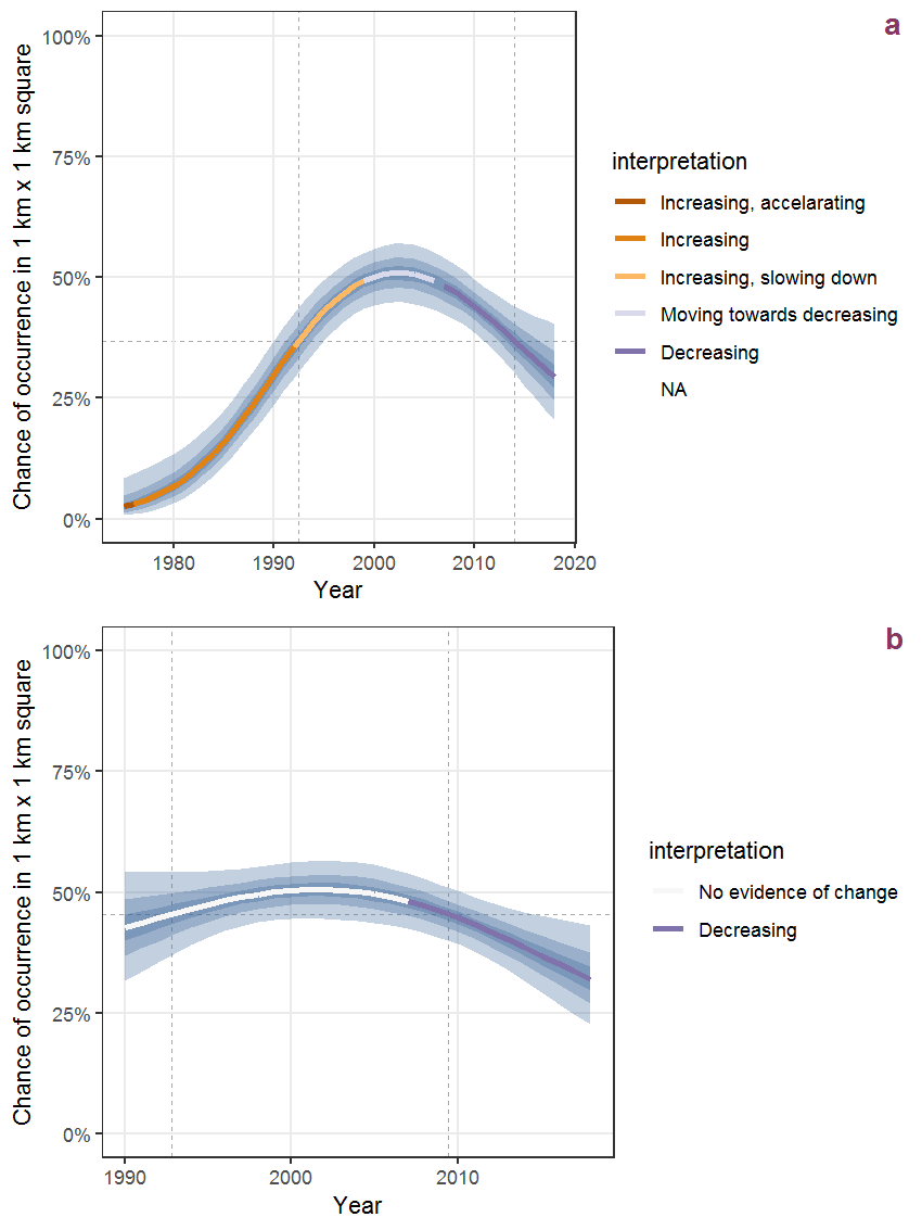
Figure B.91: Effect of year on the probability of Amaranthus hybridus L. presence in 1 km x 1 km squares where the species has been observed at least once. The fitted line shows the sum of the overall mean (the intercept), a conditional effect of list-length equal to 130 and the year-smoother. The vertical dashed lines indicate the year(s) where the year-smoother is zero. The 95% confidence band is shown in grey (including the variability around the intercept and the smoother). a: 1950 - 2018, b: 1990 - 2018.
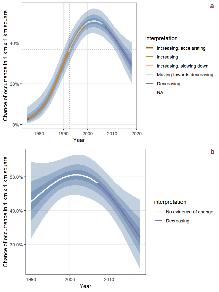
Figure B.92: The same as B.91, but the vertical axis is scaled to the range of the predicted values such that relative changes can be seen more easily. a: 1950 - 2018, b: 1990 - 2018.
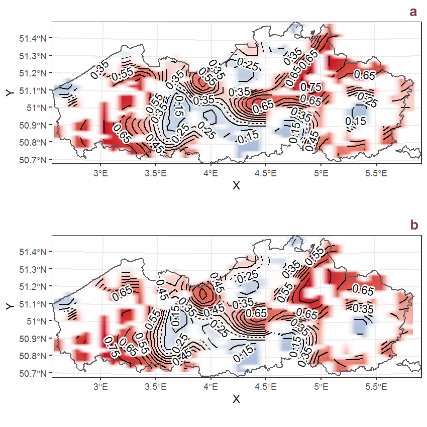
Figure B.93: Visualisation of the spatial smooth effect on the probability of Amaranthus hybridus L. presence in 1 km x 1 km squares where the species has been observed at least once. The probabilities (values on the contour lines) are conditional on the final year of observation and a list-length equal to 130. The dashed contour line demarcates zones where the species is expected to be more prevalent (red shades) from zones where the species is less prevalent (blue shades). a: 1950 - 2018, b: 1990 - 2018.
B.32 Amaranthus retroflexus L.
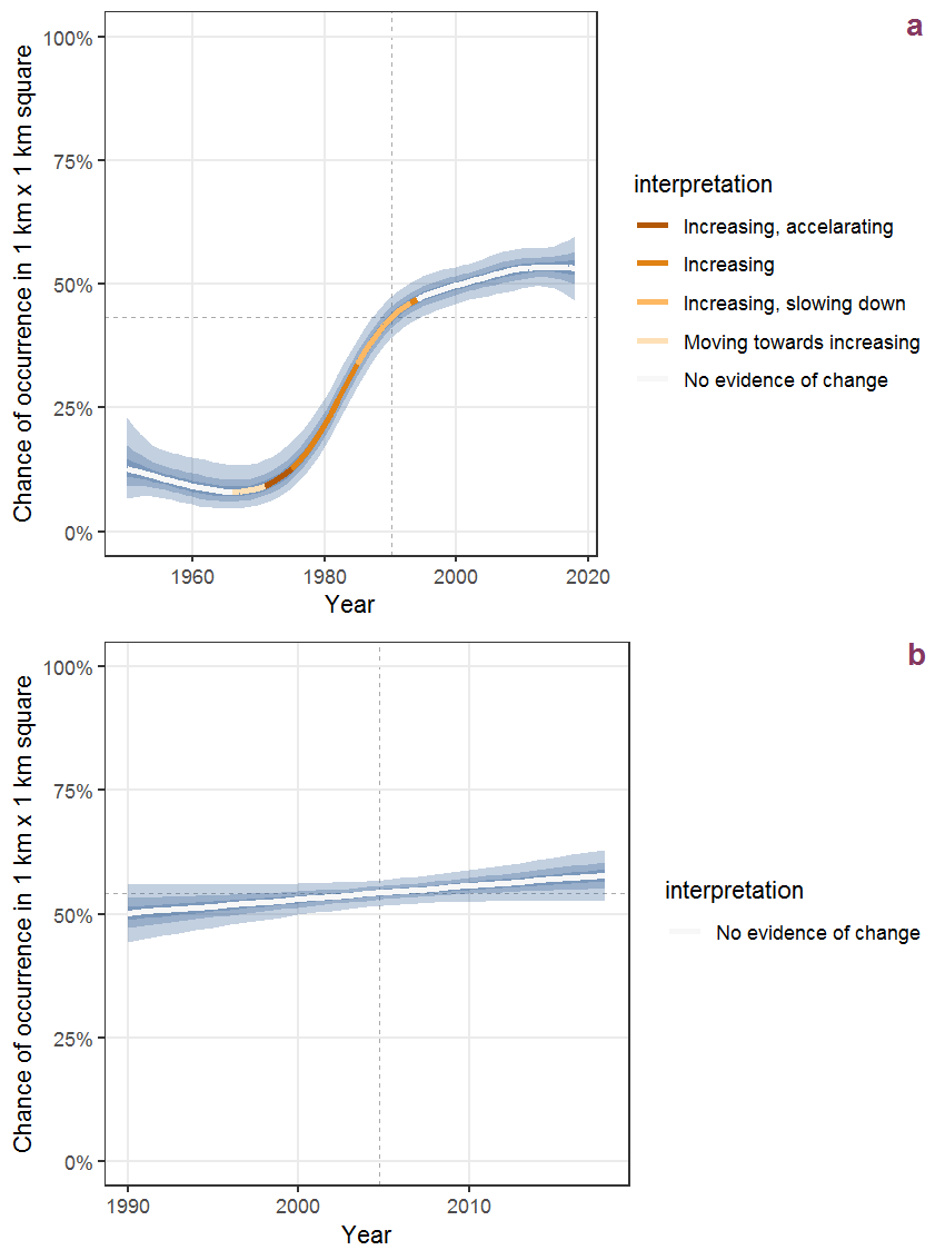
Figure B.94: Effect of year on the probability of Amaranthus retroflexus L. presence in 1 km x 1 km squares where the species has been observed at least once. The fitted line shows the sum of the overall mean (the intercept), a conditional effect of list-length equal to 130 and the year-smoother. The vertical dashed lines indicate the year(s) where the year-smoother is zero. The 95% confidence band is shown in grey (including the variability around the intercept and the smoother). a: 1950 - 2018, b: 1990 - 2018.
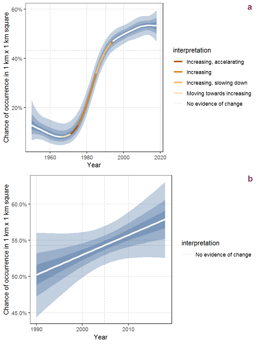
Figure B.95: The same as B.94, but the vertical axis is scaled to the range of the predicted values such that relative changes can be seen more easily. a: 1950 - 2018, b: 1990 - 2018.
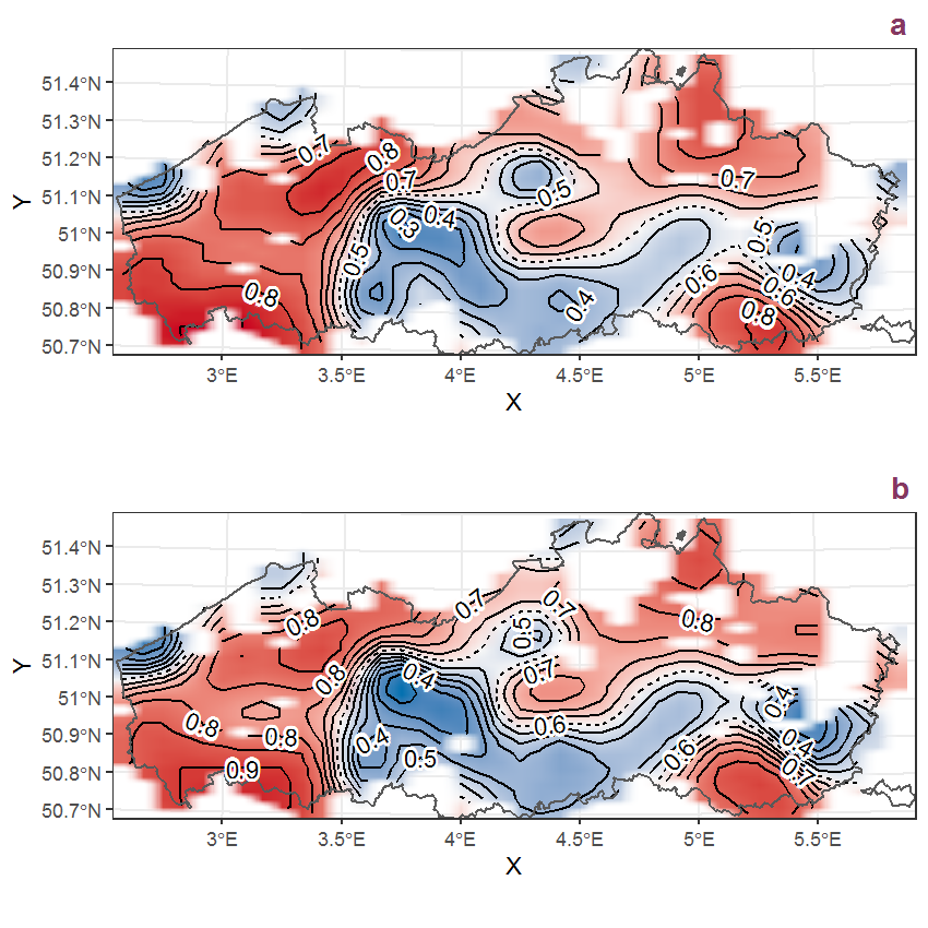
Figure B.96: Visualisation of the spatial smooth effect on the probability of Amaranthus retroflexus L. presence in 1 km x 1 km squares where the species has been observed at least once. The probabilities (values on the contour lines) are conditional on the final year of observation and a list-length equal to 130. The dashed contour line demarcates zones where the species is expected to be more prevalent (red shades) from zones where the species is less prevalent (blue shades). a: 1950 - 2018, b: 1990 - 2018.