2 Methods

2.1 Data preparation steps

2.1.1 Filter km-square-year combinations and species

The following procedure was used:

1. extract all unique combinations of 1 km x 1 km square, year (starting from 1950 or 1990) for vascular plants from the florabank (final year 2018)
2. remove 1 km x 1 km square-year combinations for which the number of species is less than or equal to n1
3. remove species for which the number of years between the first year of occurrence and the last year of occurrence is less than or equal to n2 years and the last year with occurrences is not more than n3 years ago
4. remove species for which the proportion of years with records for a species - in the period covered by the first to the last year in which a species is seen - is less than 1-in-n4
5. remove species for which the average number of 1 km x 1 km squares per year with records for the species is less than or equal to n5

with the following settings:

• n1 = 100
• n2 = 20
• n3 = 8 (i.e. 2018 - 8 = 2010)
• n4 = 3
• n5 = 10

In addition, hybrid species and aggregated taxa (species groups) were excluded from the analyses. No exclusion was made of km-squares which only partly overlap with the study region (Flanders and the Brussels capital region). In total 641 taxa were selected for further analysis.

Not all km-square-year combinations for which species records were present in the database could be considered well-surveyed. A threshold of n1 species on the list was considered as a well-surveyed square in a given year. This number was based on expert opinion as well as exploratory data analysis and was used to define absences of species from given square-year combinations, which is explained in the next section. Note that this threshold should ideally depend on characteristics of the square itself (such as the number of different vegetation types in a square, accessibility of the square, etcetera), but further research is needed to address this issue.

The number of well-surveyed km-squares per year was quite variable (see figure 2.1). In the 1950s this averaged 92 km-squares per year, but it dropped to just 30 squares per year on average in the 1960s. From the 1970s onward, the decadal average steadily increased (107, 182, 270, 276, 323 respectively).

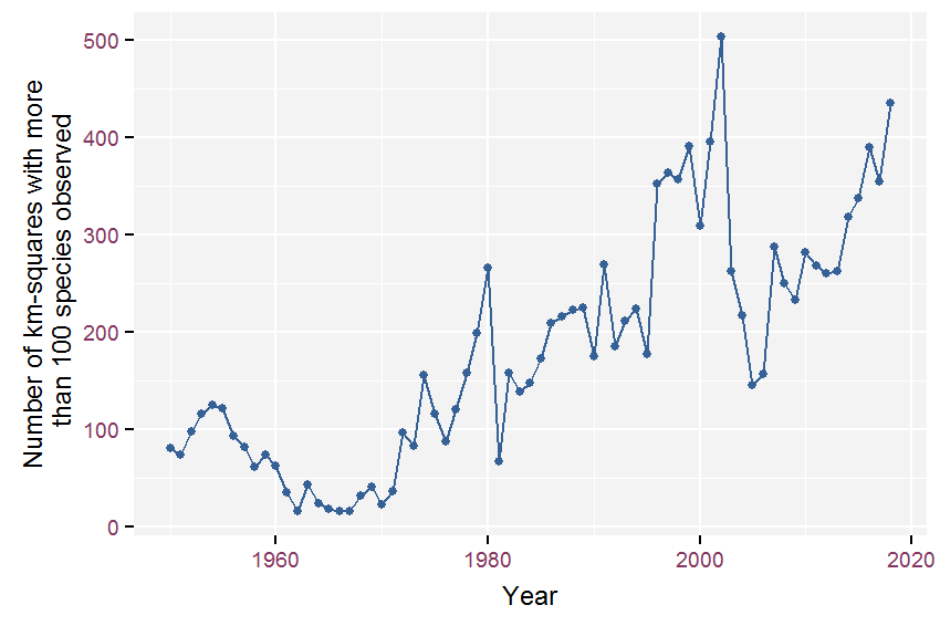
Figure 2.1: Evolution of the number of well-surveyed km-squares (list-length > 100) since 1950.

2.1.2 Procedure to generate zeroes

In a first step, we generate absences for all well-surveyed square-year combinations (i.e. more than n1 species) where the focal species was not on the list. After this first step, we obtain a dataset with the maximum number of absences. For each species this would be a dataset with an equal number of rows. These datasets would be suitable to make maps of the distribution of a species, but this is not our goal. The goal is to model occupancy trends for each species and calculate multi-species indices based on these trends.

In a second step, we therefore removed years from the beginning or the end of the time series with zero occupancy in all 1 km x 1 km squares. The main reason to do this is to avoid too wide confidence intervals when a species is absent in the begin years and only starts increasing later on (range-expanding species, invasive species), or when a species dissapears.

Third, we removed 1 km x 1 km squares with zero occupancy in all years. The reason to do this is that for species which only occur in certain parts of Flanders, for instance restricted to sandy soils, lots of zeroes are generated which has an influence on the fitted overall intercept and the spatial field. Note however that such squares may be outside as well as within the distributional range of the species.

These final presence-absence datasets (one for each species) allow us to model the species’occupancy conditionally on species’presence in a km-square in at least one year. We call this the min_zeroes_scenario.¹

2.2 Species-specific models

The presence-absence of a species (\(Y_{i,t}\)) in 1 km x 1 km square, \(i\), and year, \(t\), is modeled, through a logit-link and assuming a Bernoulli distribution, as a function of an intercept and the sum of three smoothing functions:

1. a smoothing function for year,
2. a smoothing function for space (x and y coordinates) and
3. a smoothing function for list length (the total number of species recorded in a given year and 1 km x 1 km square).

\[g(\mu_{i,t}) = \beta_0 + f_1(\text{year}_{t}) + f_2(x_{i}, y_{i}) + f_3(\text{listlength}_{i,t})\]

where

\[ \begin{aligned} \mu_{i,t} \equiv \mathbf{E}(Y_{i,t}) = P(Y_{i,t}=1)&& \text{expected value; probability of species presence}\\ g(\mu_{i,t}) = \log\frac{\mu_{i,t}}{1-\mu_{i,t}} && \text{logit-link} \\ Y_{i,t} \sim \text{Bernoulli}(\mu_{i,t}) && \text{Bernoulli distribution}\\ f_{*}(x) = \sum_{j=1}^{k}b_j(x)\beta_j && \text{smoothing function with basis } b_j \end{aligned} \]

Each smoother has a sum to zero constraint and models the deviation from the grand mean (= the intercept = \(\beta_0\)) for the considered covariate(s) in the logit-link scale. Smoothing functions are linear combinations of particular basis functions. The choice of basis function, together with the penalties applied, determine the smoothing function. Because these choices are important, we explain them for each of the smoothers in more detail.

The smoothers for year and list length are penalized thin plate regression splines. They tend to give the best mean square error performance (Wood 2017). An upper bound on the basis dimension needs to be set for these smoothers (the higher the number of basis dimensions, the wigglier the curve is allowed to be). The fitting algorithm chooses the optimal number of basis dimensions below this bound. The number of basis dimensions controls the amount of smoothing, but the resulting smooth function is not very sensitive to this choice provided that it is not too small risking oversmoothing. For year, the upper bound on the number of basis dimensions was set to one-tenth of the timespan in years for which we have observations for the species (rounded to integer). Because we expected a fairly simple relationship with list length (an increasing function), the upper bound on the number of basis dimensions was kept relatively low (set to 4).

The smoothing function for space followed the approach of a so-called generalized geo-additive model (Kammann and Wand 2003) which uses a Gaussian process basis to form the smoothing function (a.k.a. kriging). For this model a choice of covariance/correlation function needs to be made. The simplest form from the family of Matérn covariance functions was used (see Kammann and Wand (2003) for details). With this formulation two out of three parameters are fixed (a parameter that controls the smoothness - set to 3/2 - and a range parameter controlling the distances at which covariances become zero) and only the variance of the spatial process needs to be estimated. The range parameter was set to 10 (kilometer). With this setting, the correlation drops below 0.25 at a distance of 27 km (figure 2.2). The range parameter was set to a fairly short distance to focus the spatial smoothing function on short-distance correlation. This can be seen as a way to protect against type I error of the other smooths (concluding that a significant effect exists while in reality it does not) because modeling short-distance correlation accounts for dependency of 1 km x 1 km squares in close vicinity of each other (this is often the case with preferential sampling; neighboring squares are likely more similar in species composition than distant squares).

The simplified Matérn correlation function for a distance, \(d\), between two 1 km x 1 km squares, with range parameter \(\rho\) is:

\[c_0(d) = (1 + d/\rho)\exp(-d/\rho)\]

and is plotted in figure 2.2.

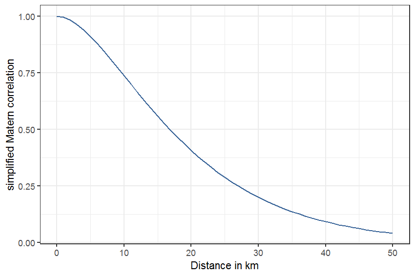
Figure 2.2: Matérn correlation function with range parameter set to 10 km.

It is possible to search for an optimal range parameter by comparing models in terms of their restricted maximum likelihood (REML) score for different values of the range parameter (Wood 2017, 362–63; Simpson 2018), but we chose a sensible setting for the range parameter over a data-driven approach. This Matérn correlation function was thus used as a basis function and the spatially smoothed pattern is a linear combination of these basis functions. The upper bound on the dimensionality of the linear combination was defined as the minimum of 100 and the number of unique locations (1 km x 1 km squares) in the analysis dataset for the species.

The above model formulation was thus applied to each species for which enough data were available (see section 2.1). The amount of smoothing (in space, in time, and for list-length) will be different for each species and will be chosen in a data-driven way based on optimization of the REML scores (with upper bounds as explained above). All species models were run using a dataset spanning 1950 - 2018 and a dataset spanning 1990 - 2018.

The models did not include an offset term to account for differences in the size of overlap between the study region and the km-square. About 84% of km-squares are situated completely within the study region. However, even in such squares, accessibility can be as low as 5% (for instance, industrial areas, or agricultural areas with few roads). Conversely, a km-square that overlaps only 10% with the study area, could be very accessible. Data on accessibility for each km-square were not available, but should be considered in future research.

2.3 Multi-species index

2.3.1 Calculation

An index represents a change from one value to another (baseline) value. A multi-species index combines indices from multiple species in a single index of change.

Following Buckland et al. (2011) we can calculate the geometric mean of “relative abundances” (which equals the backtransformed arithmetic mean of log-transformed relative abundances). Relative abundance in terms of species prevalence is equivalent to the proportion of a species in a year divided by the proportion of the same species in a chosen baseline year. This ratio of proportions is also called a relative risk in medicine (risk because of risk of disease, but that would be a misnomer in our context). The same rationale is behind the so-called response ratio in meta-analysis literature (Lajeunesse 2011).

\[\begin{align*} \hat\pi_{j,t} = \frac{\exp(\hat{l_{j,t}})}{1 + \exp(\hat{l_{j,t}})}\\ \text{SI}_{j,t} = \frac{\hat\pi_{j,t}}{\hat\pi_{j,baseline}}\\ \text{MSI}_{t} = 100\times \exp\bigg( \frac{1}{s}\sum_{j = 1}^{s}\log\text{SI}_{j,t}\bigg)\\ \text{SE}_{\text{MSI}} = \sqrt{\frac{1}{s}\sum_{j = 1}^{s}\text{SE}_{\text{SI}}^2}\\ \end{align*}\]

In these formulas, \(j\) indexes species, \(t\) indexes years, \(l\) is the linear predictor in the logit scale and \(s\) is the total number of species. \(\text{MSI}\) and \(\text{SI}\) are abbreviations for multi-species index and species index, respectively. \(\text{SE}\) is the standard error.

In order not to complicate the calculation too much, we assume that each species is independent. The standard error for the multi-species index can then be calculated as the square-root of the mean of the squared standard errors of the species indices. The standard error of the species indices can be approximated by formulae assuming asymptotic normality of the logged-values (see e.g. Agresti 2002), but a better approach for these derived quantities, that are a non-linear function of the model coefficients, is to simulate from the posterior distribution of the model (Wood 2017, 293).² Using these simulations, we can calculate standard errors and Bayesian (95%) credible intervals. Although these are Bayesian credible intervals, they have very good frequentist coverage properties (Wood 2017), which means we can just as well call them 95% confidence intervals.

In some cases (broad habitat preferences, substrate, Ellenberg values and CSR values), the MSI will be calculated as a weighted mean (see section 2.4.1). Species-specific weights then represent how much each species should contribute in the calculation of the mean relative to the other species. Weighting can either be done using the numerical values of a numerical species trait, or, within a category of a categorical species trait. For instance, Ellenberg values (for soil fertility (N), soil or water acidity (R), temperature (T), or soil moisture (F)) and CSR ordinate values (indicating degree of competitiveness (C), or stress-tolerance (S), or ruderalism (R)) can be used at face value as weights. Or, they can be reclassified into a small number of classes to aid interpretability. Within each class, the recoded Ellenberg values can be used to weigh species belonging to that class. For instance, within a broad class of “species indicating acid conditions”, species with Ellenberg values indicating very acid conditions will receive more weight than species indicating acid conditions.

2.3.2 Guidelines for statistical interpretation

For the species-indices and multi-species indices, differences between years can only be judged relative to the baseline year. As a consequence, every year needs to be taken as a baseline in order to be able to assess differences between any two years. The figures showing the MSIs as a function of year, use the year 2000 as baseline year (see results 3). Confidence intervals (95% confidence level) aid to assess if the index in a given year is significantly different from the year 2000.

To further help with the (statistical) interpretation of the multi-species indices, each figure of a multi-species index (showing the index values relative to baseline year 2000) will be accompanied by (1) an interpretation of the temporal changes based on the rate of change and the acceleration of the change in a given year, and (2) a side panel and a table showing, respectively, how many and which plant species have changed and by how much when the final year is compared to the first year. We explain both cases in the following paragraphs.

Fewster et al. (2000), Buckland et al. (2011) and Harrison et al. (2014) calculate the first and second derivative of the multi-species index smoothed trend. Importantly, these derivatives are independent of the chosen baseline. The first derivative is the speed of change in the trend. The second derivative is the change in the speed of change in the trend and can be useful to assess compliance with some biodiversity targets. For instance the 2010 target was formulated as a “significant reduction in the current rate of biodiversity loss”). These derivatives, together with their 95% confidences intervals, allow us to classify the trend as shown in table 2.1. The same approach and classification is also used in the plots showing the trends for individual species.

Table 2.1: Interpretation of the trend based on the first (rate of change) and second derivative (acceleration) of the smoother for year.

We used a detailed classification to assess a \(SI\) comparing the last year of observation against the first year of observation (= new baseline). This classification is based entirely on the location of the 95% confidence interval around this species index with respect to the reference (i.e. \(SI = 1\) indicating no change) and an upper (\(4/3\)) and a lower threshold (\(3/4\)). These thresholds are used to discern between the strength of trends. The resulting classification is shown in Table 2.2.

Table 2.2: Classification used to evaluate a species index where the last year is compared to the first year

Symbol	Trend	Location of confidence interval
++	strong increase	above the upper threshold
+	increase	above reference and contains the upper threshold
+~	moderate increase	between reference and the upper threshold
~	stable	between thresholds and contains reference
-~	moderate decrease	between reference and the lower threshold
-	decrease	below reference and contains the lower threshold
–	strong decrease	below the lower threshold
?+	potential increase	contains reference and the upper threshold
?-	potential decrease	contains reference and the lower threshold
?	unknown	contains the lower and upper threshold

Two versions of all multi-species indices were calculated: one based on the 1950 - 2018 species models, and another based on the 1990 - 2018 species models. It was possible that species models had model predictions that did not cover the entire period, because the species was observed for the first time well past the first year of the considered period. The reverse, a species disappearing well before the final year was never the case (this is only due to the stringent data requirements which rule out rare species which have a higher extinction risk). No attempt was made to correct the multi-species indices for these years without predictions (although procedures exist that do this, see Soldaat et al. (2017)). Instead these species were removed from the calculation of the multi-species indices, so that any bias that could result from including these species is avoided. This implies that the multi-species indices for the period 1950 - 2018 are based on fewer species than the multi-species indices for the period 1990 - 2018. The benefit of considering the 1950 - 2018 period is that the multi-species indices can show a long-term picture of change - less prone to issues of shifting baseline (Soga and Gaston 2018) - while the 1990 - 2018 multi-species indices are more robust because they focus on a time frame where more data for more species are available.

2.4 Considered species groups

2.4.1 Weighting schemes

Some species groups were derived from ecotope types as published in Runhaar et al. (2004). Ecotopes were defined in that publication as a spatial unit that is homogeneous with regard to vegetation structure and factors that determine plant growth.

For species groups that were derived from ‘ecotopes’ (see Runhaar et al. 2004), i.e. a clustering of ecotopes in broader habitat groups, a clustering indicating nutrient availability and a clustering of ecotopes in substrate classes, a weighted MSI was calculated. The reason we use weights here is that a species can occur in multiple ecotopes; a species can thus be very restricted to a single ecotope or, conversely, occur in multiple ecotopes. The weight for each species was determined as the number of ecotopes within a given habitat group or substrate class where the species can occur divided by the total number of ecotopes where the species can occur.

For species where a CSR type (Competitiveness, Stress-tolerance and Ruderality) was available, each species was given a weight for each of the three dimensions (C, S and R) according to table 2.3.

Table 2.3: Translation of CSR-types to degrees of competitiveness (C), stress-tolerance (S) and ruderalism (R).

csr_type	C	S	R
C	1.00	0.00	0.00
C/CR	0.75	0.00	0.25
C/CSR	0.67	0.17	0.17
C/SC	0.75	0.25	0.00
CR	0.50	0.00	0.50
CR/CSR	0.42	0.17	0.42
CSR	0.33	0.33	0.33
R	0.00	0.00	1.00
R/CR	0.25	0.00	0.75
R/CSR	0.17	0.17	0.67
R/SR	0.00	0.25	0.75
S	0.00	1.00	0.00
S/CSR	0.17	0.67	0.17
S/SC	0.25	0.75	0.00
S/SR	0.00	0.75	0.25
SC	0.50	0.50	0.00
SC/CSR	0.42	0.42	0.17
SR	0.00	0.50	0.50
SR/CSR	0.17	0.42	0.42

Table 2.4 shows the weights that are used to calculate multi-species indices based on Ellenberg indicator values. Two variants were considered. For the first variant, the multi-species indices were calculated based on the species belonging to the grouping defined by the column ‘Description’. In this case, the weights in the ‘Weights’ column were used to calculated a weighted MSI. For the second variant, the weighted multi-species indices were calculated based on the grouping defined by the column ‘Ellenberg_indicator’ and using weights defined in the column ‘Ellenberg_value’ (the original Ellenberg values). As an example, in the latter case, gradually more weight will be given to species indicative of increasingly basic soils when calculating the weighted MSI for Ellenberg R (reaction number).

Table 2.4: Weighting schemes used for the regrouped Ellenberg indicators.

Description	Ellenberg_indicator	Ellenberg_value	Weight
dry	Ellenberg humidity value (regrouped)	2	4
dry	Ellenberg humidity value (regrouped)	3	3
dry	Ellenberg humidity value (regrouped)	4	2
dry	Ellenberg humidity value (regrouped)	5	1
moist	Ellenberg humidity value (regrouped)	6	1
moist	Ellenberg humidity value (regrouped)	7	1
wet	Ellenberg humidity value (regrouped)	8	1
wet	Ellenberg humidity value (regrouped)	9	2
temporarilly submerged	Ellenberg humidity value (regrouped)	10	1
submerged	Ellenberg humidity value (regrouped)	11	1
submerged	Ellenberg humidity value (regrouped)	12	1
nitrogen deprived	Ellenberg nitrogen value (regrouped)	1	3
nitrogen deprived	Ellenberg nitrogen value (regrouped)	2	2
nitrogen deprived	Ellenberg nitrogen value (regrouped)	3	1
nitrogen intermediat	Ellenberg nitrogen value (regrouped)	4	1
nitrogen intermediat	Ellenberg nitrogen value (regrouped)	5	1
nitrogen intermediat	Ellenberg nitrogen value (regrouped)	6	1
nitrogen rich	Ellenberg nitrogen value (regrouped)	7	1
nitrogen rich	Ellenberg nitrogen value (regrouped)	8	2
nitrogen rich	Ellenberg nitrogen value (regrouped)	9	3
acidic	Ellenberg reaction value (regrouped)	1	3
acidic	Ellenberg reaction value (regrouped)	2	2
acidic	Ellenberg reaction value (regrouped)	3	1
weakly acidic	Ellenberg reaction value (regrouped)	4	1
weakly acidic	Ellenberg reaction value (regrouped)	5	1
weakly acidic	Ellenberg reaction value (regrouped)	6	1
weakly basic or basic	Ellenberg reaction value (regrouped)	7	1
weakly basic or basic	Ellenberg reaction value (regrouped)	8	2
weakly basic or basic	Ellenberg reaction value (regrouped)	9	3
cool	Ellenberg temperature value (regrouped)	3	2
cool	Ellenberg temperature value (regrouped)	4	1
moderate	Ellenberg temperature value (regrouped)	5	1
moderate	Ellenberg temperature value (regrouped)	6	1
warm	Ellenberg temperature value (regrouped)	7	1
warm	Ellenberg temperature value (regrouped)	8	2

2.4.2 Overview

Table 2.5 gives an overview of all species groups and traits that were considered for calculation of group- or trait-specific MSI.

Table 2.5: Overview of all species traits.

Table 2.6 is a species by species trait table, which allows - for instance - to filter for species which are classified as “warm”, according to Ellenberg temperature and “neophyte” (column indigeneous, archeophyte or neophyte).

Table 2.6: Overview of all species together with information for each trait.

2.5 Computational reproducibility

All analysis were executed using the R software for statistical programming. The scripts for these analyses are under Git version control and are deposited on a private GitHub repository.

The species models were run in a separate analysis pipeline using R version 3.6.1 and the following R package versions:

Package	Version
BH	1.69.0-1
DBI	1.0.0
Formula	1.2-3
KernSmooth	2.23-15
MASS	7.3-51.4
Matrix	1.2-17
R6	2.4.1
RColorBrewer	1.1-2
RCurl	1.95-4.12
RSQLite	2.1.1
Rcpp	1.0.3
askpass	1.1
assertable	0.2.5
assertthat	0.2.1
backports	1.1.5
base64enc	0.1-3
base64url	1.4
bit	1.1-14
bit64	0.9-7
bitops	1.0-6
blob	1.2.0
checkmate	1.9.4
class	7.3-15
classInt	0.3-3
cli	2.0.0
clipr	0.6.0
codetools	0.2-16
colorspace	1.4-1
cowplot	1.0.0
crayon	1.3.4
crosstalk	1.0.0
crul	0.8.0
curl	4.3
data.table	1.12.2
digest	0.6.23
dotCall64	1.0-0
dplyr	0.8.3
drake	7.8.0
e1071	1.7-2
effectclass	0.1.1
ellipsis	0.3.0
fansi	0.4.0
farver	2.0.1
fields	9.8-3
filelock	1.0.2
foreign	0.8-71
formula.tools	1.7.1
future	1.14.0
geoaxe	0.1.0
ggplot2	3.2.1
globals	0.12.4
glue	1.3.1
gratia	0.2-8
gridExtra	2.3
gtable	0.3.0
hms	0.5.0
htmltools	0.3.6
htmlwidgets	1.3
httpcode	0.2.0
httpuv	1.5.1
httr	1.4.0
igraph	1.2.4.2
inborutils	0.1.0.9072
iterators	1.0.10
jsonlite	1.6
labeling	0.3
later	0.8.0
lattice	0.20-38
lazyeval	0.2.2
leaflet	2.0.2
lifecycle	0.1.0
listenv	0.7.0
lubridate	1.7.4
magrittr	1.5
maps	3.3.0
maptools	0.9-5
markdown	1.1
memoise	1.1.0
metR	0.4.0
mgcv	1.8-28
mime	0.7
munsell	0.5.0
mvtnorm	1.0-11
nlme	3.1-140
oai	0.2.2
odbc	1.1.6
openssl	1.4
operator.tools	1.6.3
pillar	1.4.3
pkgconfig	2.0.3
plogr	0.2.0
plyr	1.8.5
png	0.1-7
prettyunits	1.0.2
promises	1.0.1
purrr	0.3.3
raster	2.9-23
readr	1.3.1
renv	0.9.3-23
reshape2	1.4.3
rgbif	1.3.0
rgdal	1.4-4
rgeos	0.4-3
rlang	0.4.2
rootSolve	1.7
rprojroot	1.3-2
scales	1.1.0
sf	0.7-6
shiny	1.3.2
sourcetools	0.1.7
sp	1.3-1
spam	2.2-2
storr	1.2.1
stringi	1.4.3
stringr	1.4.0
sys	3.2
tibble	2.1.3
tidyr	1.0.0
tidyselect	0.2.5
triebeard	0.3.0
txtq	0.2.0
units	0.6-3
urltools	1.7.3
utf8	1.1.4
vctrs	0.2.1
viridis	0.5.1
viridisLite	0.3.0
visNetwork	2.0.7
whisker	0.3-2
wicket	0.4.0
withr	2.1.2
xfun	0.8
xml2	1.2.0
xtable	1.8-4
yaml	2.2.0
zeallot	0.1.0

The multi-species indices are calculated as part of this technical report, which is written as a bookdown / R markdown report (combining text and R scripting). For this report, the following version of R and versions of R packages are used:

R version 4.0.2 (2020-06-22)

Platform: x86_64-w64-mingw32/x64 (64-bit)

locale: LC_COLLATE=Dutch_Belgium.1252, LC_CTYPE=Dutch_Belgium.1252, LC_MONETARY=Dutch_Belgium.1252, LC_NUMERIC=C and LC_TIME=Dutch_Belgium.1252

attached base packages:

• stats
• graphics
• grDevices
• utils
• datasets
• methods
• base

other attached packages:

• gratia(v.0.4.1)
• metR(v.0.7.0)
• scales(v.1.1.1)
• rootSolve(v.1.8.2.1)
• effectclass(v.0.1.3)
• mgcv(v.1.8-33)
• nlme(v.3.1-149)
• cowplot(v.1.1.0)
• sf(v.0.9-5)
• rprojroot(v.1.3-2)
• inbodb(v.0.0.0.9000)
• INBOtheme(v.0.5.6)
• forcats(v.0.5.0)
• stringr(v.1.4.0)
• dplyr(v.1.0.2)
• purrr(v.0.3.4)
• readr(v.1.3.1)
• tidyr(v.1.1.2)
• tibble(v.3.0.3)
• ggplot2(v.3.3.2)
• tidyverse(v.1.3.0)
• drake(v.7.12.5)
• knitr(v.1.30)

loaded via a namespace (and not attached):

• fs(v.1.5.0)
• lubridate(v.1.7.9)
• bit64(v.4.0.5)
• filelock(v.1.0.2)
• INBOmd(v.0.4.7)
• progress(v.1.2.2)
• httr(v.1.4.2)
• tools(v.4.0.2)
• backports(v.1.1.9)
• DT(v.0.15)
• R6(v.2.4.1)
• KernSmooth(v.2.23-17)
• DBI(v.1.1.0)
• colorspace(v.1.4-1)
• withr(v.2.2.0)
• tidyselect(v.1.1.0)
• prettyunits(v.1.1.1)
• rematch(v.1.0.1)
• bit(v.4.0.4)
• compiler(v.4.0.2)
• cli(v.2.0.2)
• rvest(v.0.3.6)
• xml2(v.1.3.2)
• labeling(v.0.3)
• bookdown(v.0.21)
• checkmate(v.2.0.0)
• classInt(v.0.4-3)
• odbc(v.1.2.3)
• mvnfast(v.0.2.5)
• digest(v.0.6.25)
• txtq(v.0.2.3)
• rmarkdown(v.2.4)
• R.utils(v.2.10.1)
• pkgconfig(v.2.0.3)
• htmltools(v.0.5.0)
• highr(v.0.8)
• dbplyr(v.1.4.4)
• htmlwidgets(v.1.5.1)
• rlang(v.0.4.8)
• readxl(v.1.3.1)
• rstudioapi(v.0.11)
• farver(v.2.0.3)
• generics(v.0.0.2)
• jsonlite(v.1.7.1)
• crosstalk(v.1.1.0.1)
• R.oo(v.1.24.0)
• magrittr(v.1.5)
• patchwork(v.1.0.1)
• Matrix(v.1.2-18)
• Rcpp(v.1.0.5)
• munsell(v.0.5.0)
• fansi(v.0.4.1)
• lifecycle(v.0.2.0)
• R.methodsS3(v.1.8.1)
• stringi(v.1.5.3)
• yaml(v.2.2.1)
• storr(v.1.2.1)
• grid(v.4.0.2)
• blob(v.1.2.1)
• parallel(v.4.0.2)
• crayon(v.1.3.4)
• lattice(v.0.20-41)
• haven(v.2.3.1)
• qrcode(v.0.1.2)
• splines(v.4.0.2)
• pander(v.0.6.3)
• hms(v.0.5.3)
• pillar(v.1.4.6)
• igraph(v.1.2.5)
• base64url(v.1.4)
• reprex(v.0.3.0)
• glue(v.1.4.2)
• evaluate(v.0.14)
• data.table(v.1.13.0)
• modelr(v.0.1.8)
• vctrs(v.0.3.4)
• cellranger(v.1.1.0)
• gtable(v.0.3.0)
• assertthat(v.0.2.1)
• xfun(v.0.18)
• broom(v.0.7.0)
• e1071(v.1.7-3)
• class(v.7.3-17)
• units(v.0.6-7)
• ellipsis(v.0.3.1)
• here(v.0.1)

---

1. In an exploratory phase, we also explored the effect of several alternative data preparation scenarios on the model outcomes. We added 1 km x 1 km squares in which the species had not been recorded in any of the years, but which were within a unioned polygon obtained by a buffer distance surrounding the points in the min_zeroes_scenario and disregarded the squares which were inside an inner buffer distance applied to the unioned polygon. Different combinations of outer and inner buffer distances were tried but the min_zeroes_scenario was deemed best.↩︎

2. it can be shown that the smoothers - although calculated using frequentist methodology - can be viewed from a Bayesian perspective↩︎