R Sagina apetala Ard. - Senecio sylvaticus L.
R.1 Sagina apetala Ard.
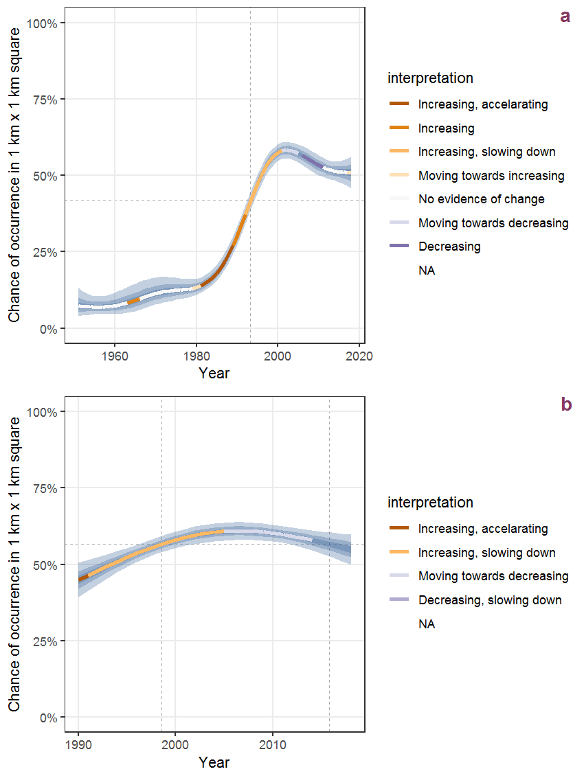
Figure R.1: Effect of year on the probability of Sagina apetala Ard. presence in 1 km x 1 km squares where the species has been observed at least once. The fitted line shows the sum of the overall mean (the intercept), a conditional effect of list-length equal to 130 and the year-smoother. The vertical dashed lines indicate the year(s) where the year-smoother is zero. The 95% confidence band is shown in grey (including the variability around the intercept and the smoother). a: 1950 - 2018, b: 1990 - 2018.
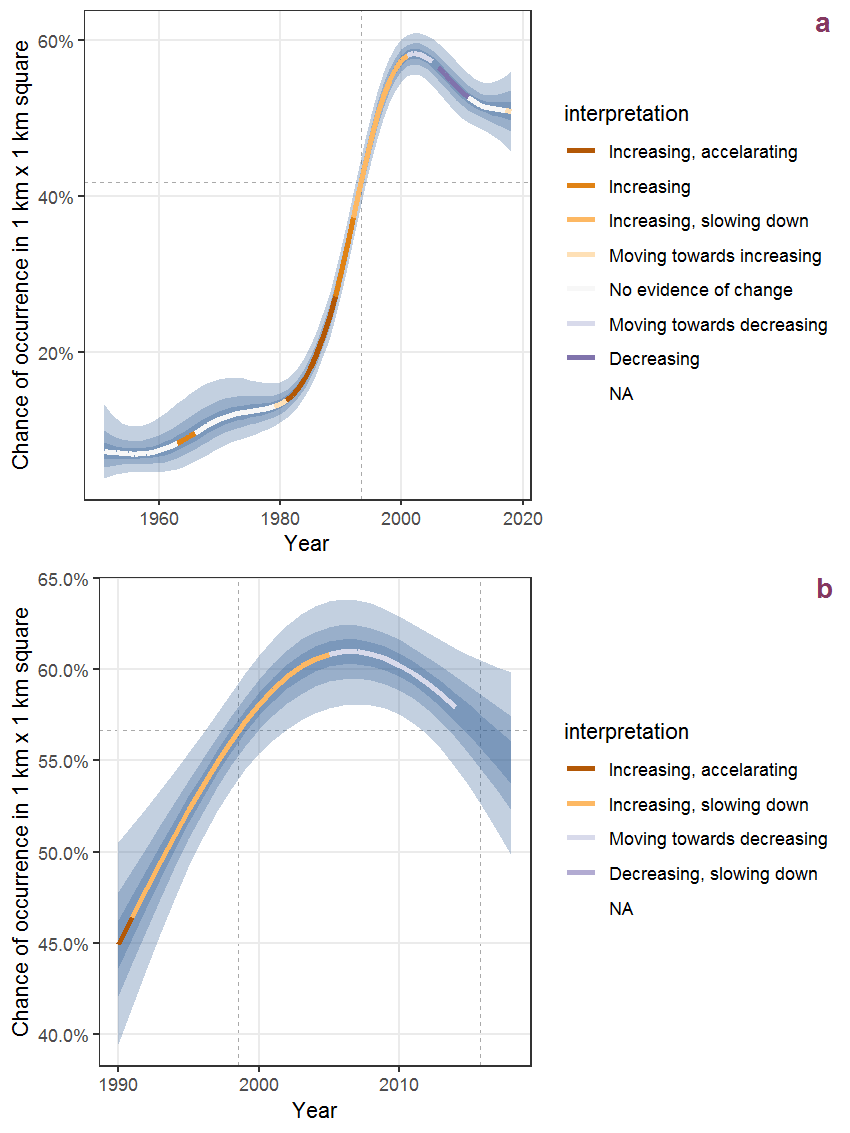
Figure R.2: The same as R.1, but the vertical axis is scaled to the range of the predicted values such that relative changes can be seen more easily. a: 1950 - 2018, b: 1990 - 2018.
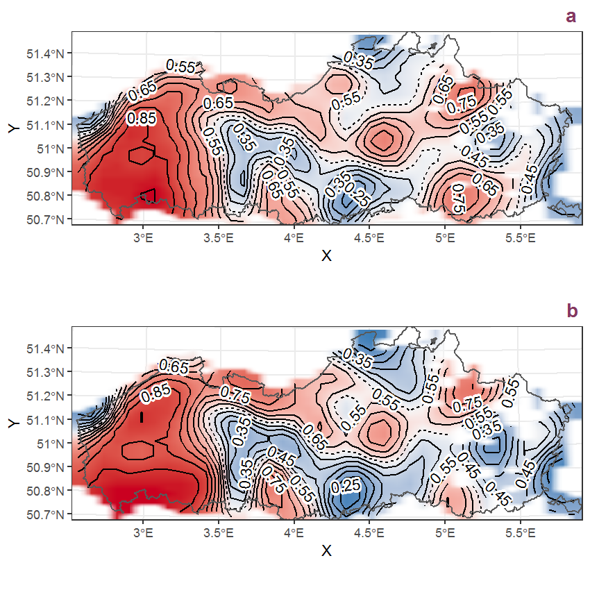
Figure R.3: Visualisation of the spatial smooth effect on the probability of Sagina apetala Ard. presence in 1 km x 1 km squares where the species has been observed at least once. The probabilities (values on the contour lines) are conditional on the final year of observation and a list-length equal to 130. The dashed contour line demarcates zones where the species is expected to be more prevalent (red shades) from zones where the species is less prevalent (blue shades). a: 1950 - 2018, b: 1990 - 2018.
R.2 Sagina procumbens L.
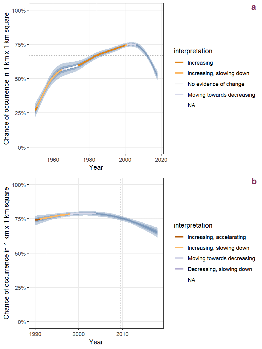
Figure R.4: Effect of year on the probability of Sagina procumbens L. presence in 1 km x 1 km squares where the species has been observed at least once. The fitted line shows the sum of the overall mean (the intercept), a conditional effect of list-length equal to 130 and the year-smoother. The vertical dashed lines indicate the year(s) where the year-smoother is zero. The 95% confidence band is shown in grey (including the variability around the intercept and the smoother). a: 1950 - 2018, b: 1990 - 2018.
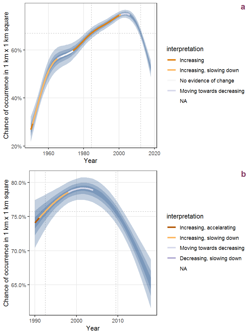
Figure R.5: The same as R.4, but the vertical axis is scaled to the range of the predicted values such that relative changes can be seen more easily. a: 1950 - 2018, b: 1990 - 2018.
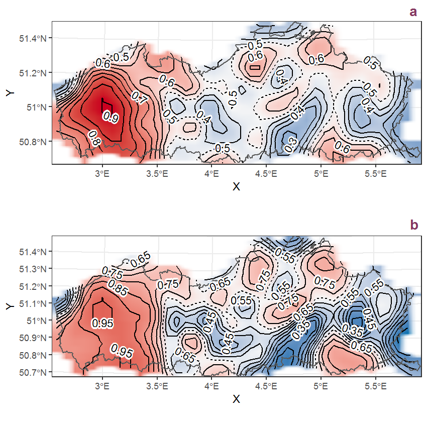
Figure R.6: Visualisation of the spatial smooth effect on the probability of Sagina procumbens L. presence in 1 km x 1 km squares where the species has been observed at least once. The probabilities (values on the contour lines) are conditional on the final year of observation and a list-length equal to 130. The dashed contour line demarcates zones where the species is expected to be more prevalent (red shades) from zones where the species is less prevalent (blue shades). a: 1950 - 2018, b: 1990 - 2018.
R.3 Sagittaria sagittifolia L.
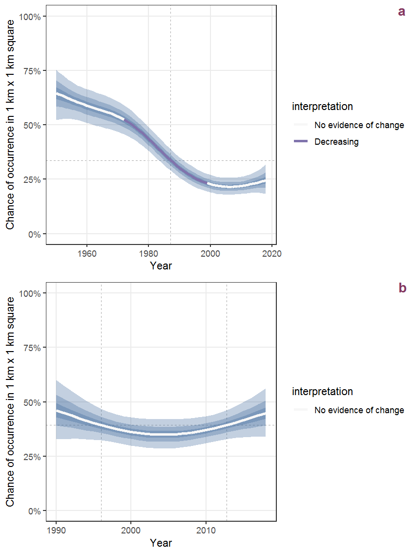
Figure R.7: Effect of year on the probability of Sagittaria sagittifolia L. presence in 1 km x 1 km squares where the species has been observed at least once. The fitted line shows the sum of the overall mean (the intercept), a conditional effect of list-length equal to 130 and the year-smoother. The vertical dashed lines indicate the year(s) where the year-smoother is zero. The 95% confidence band is shown in grey (including the variability around the intercept and the smoother). a: 1950 - 2018, b: 1990 - 2018.
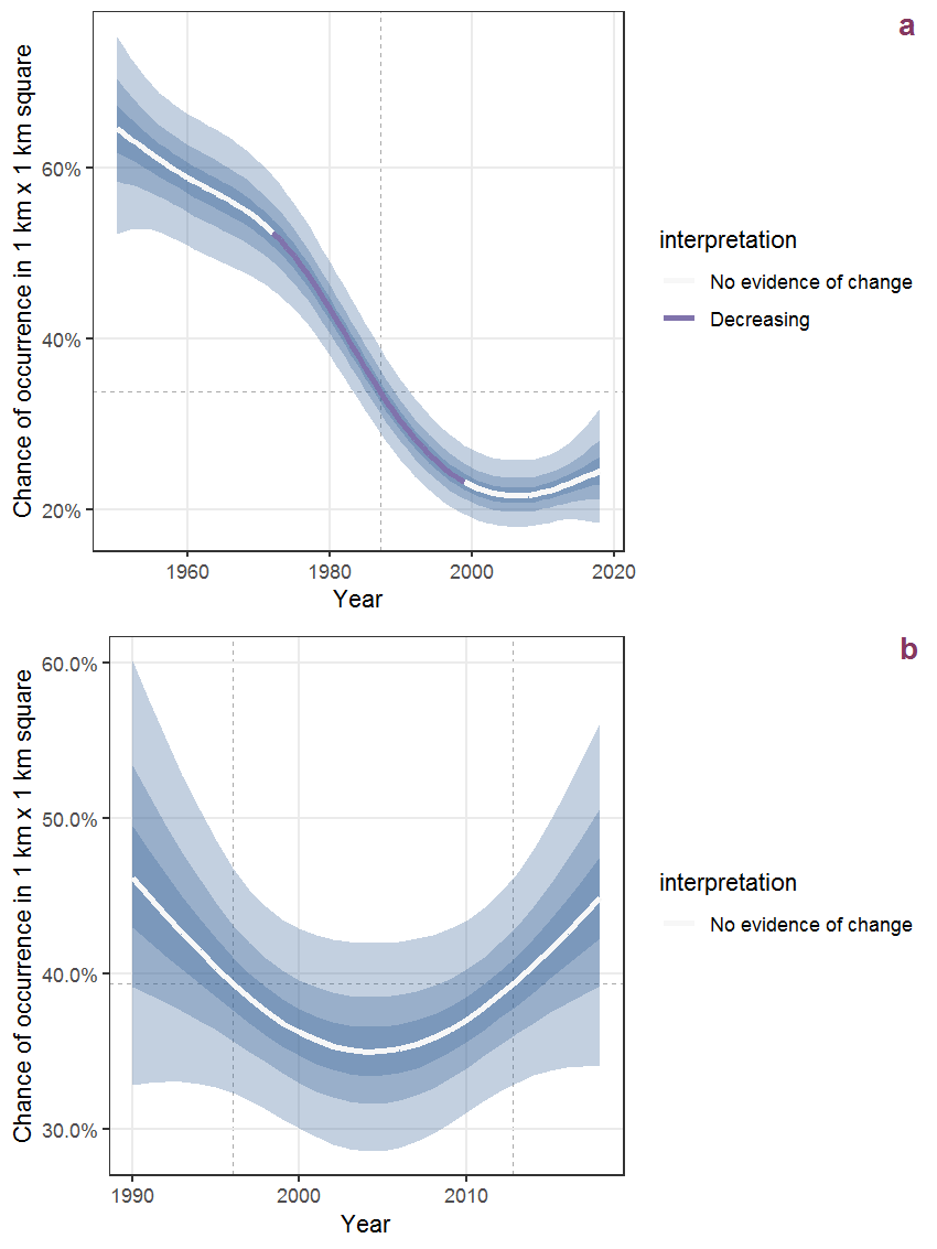
Figure R.8: The same as R.7, but the vertical axis is scaled to the range of the predicted values such that relative changes can be seen more easily. a: 1950 - 2018, b: 1990 - 2018.
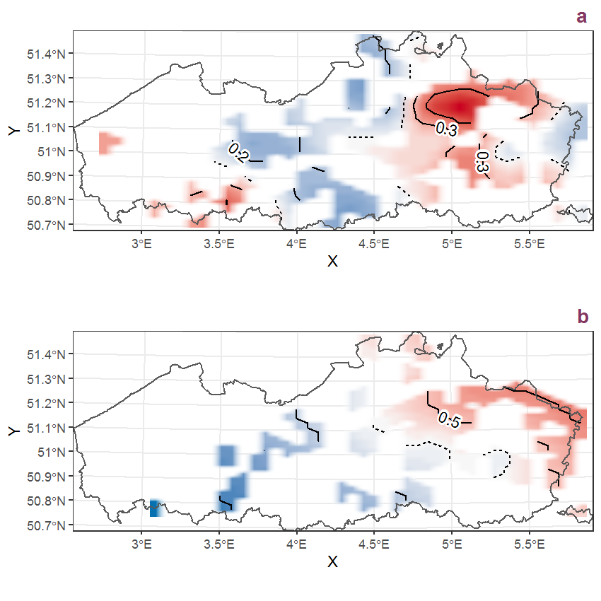
Figure R.9: Visualisation of the spatial smooth effect on the probability of Sagittaria sagittifolia L. presence in 1 km x 1 km squares where the species has been observed at least once. The probabilities (values on the contour lines) are conditional on the final year of observation and a list-length equal to 130. The dashed contour line demarcates zones where the species is expected to be more prevalent (red shades) from zones where the species is less prevalent (blue shades). a: 1950 - 2018, b: 1990 - 2018.
R.4 Salix alba L.
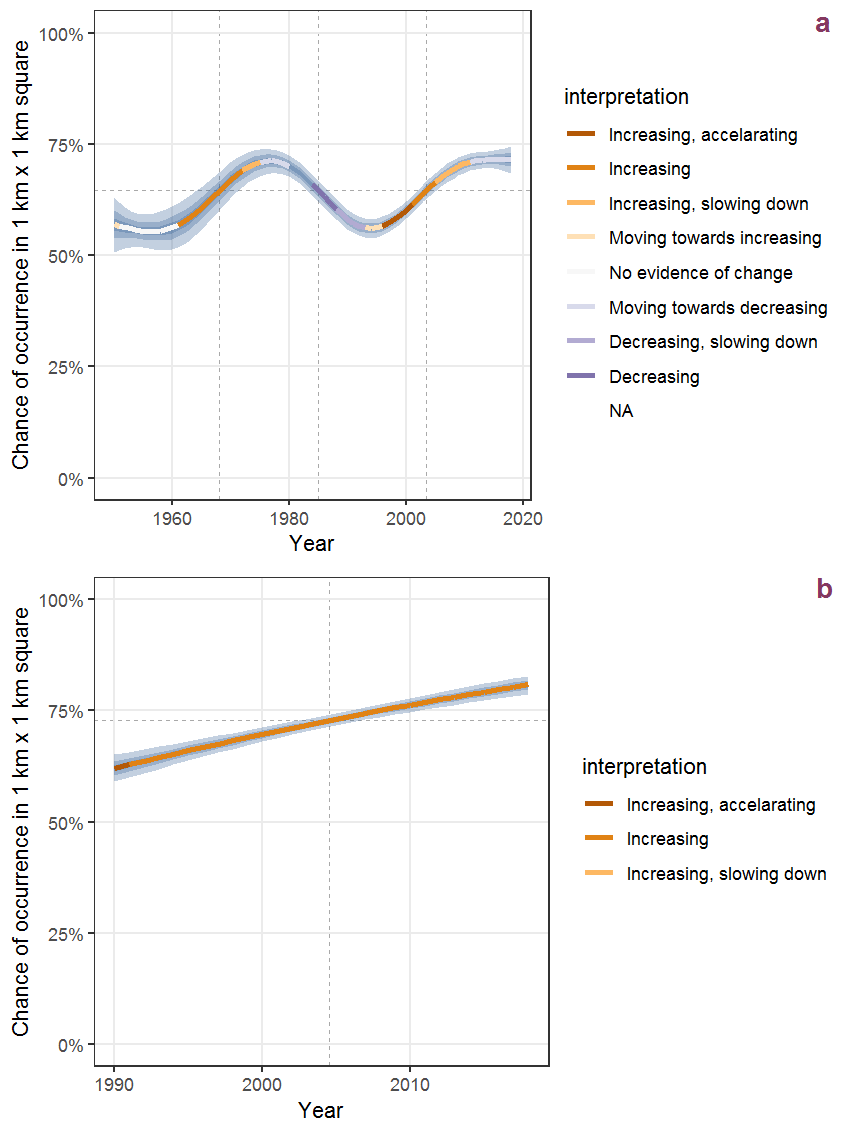
Figure R.10: Effect of year on the probability of Salix alba L. presence in 1 km x 1 km squares where the species has been observed at least once. The fitted line shows the sum of the overall mean (the intercept), a conditional effect of list-length equal to 130 and the year-smoother. The vertical dashed lines indicate the year(s) where the year-smoother is zero. The 95% confidence band is shown in grey (including the variability around the intercept and the smoother). a: 1950 - 2018, b: 1990 - 2018.
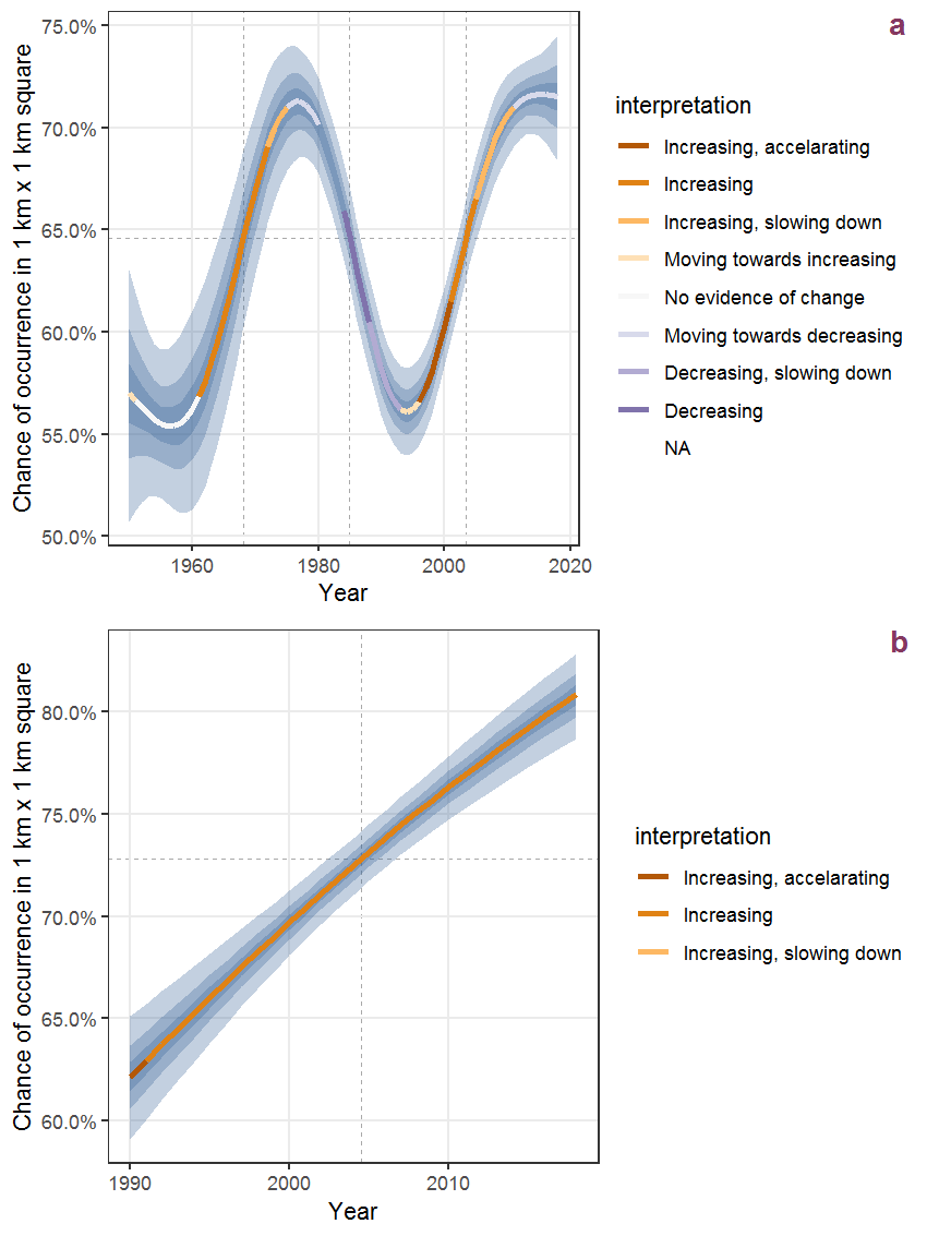
Figure R.11: The same as R.10, but the vertical axis is scaled to the range of the predicted values such that relative changes can be seen more easily. a: 1950 - 2018, b: 1990 - 2018.
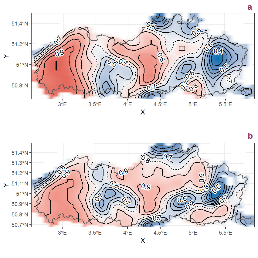
Figure R.12: Visualisation of the spatial smooth effect on the probability of Salix alba L. presence in 1 km x 1 km squares where the species has been observed at least once. The probabilities (values on the contour lines) are conditional on the final year of observation and a list-length equal to 130. The dashed contour line demarcates zones where the species is expected to be more prevalent (red shades) from zones where the species is less prevalent (blue shades). a: 1950 - 2018, b: 1990 - 2018.
R.5 Salix aurita L.
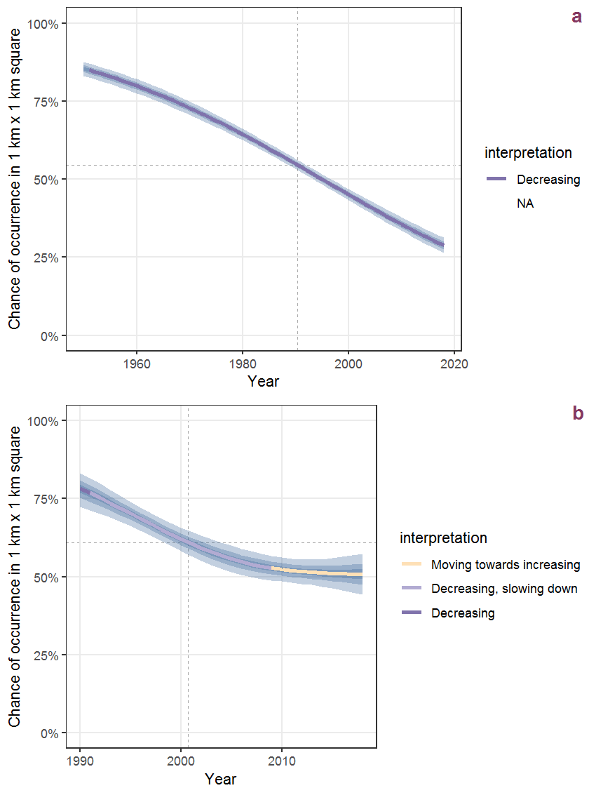
Figure R.13: Effect of year on the probability of Salix aurita L. presence in 1 km x 1 km squares where the species has been observed at least once. The fitted line shows the sum of the overall mean (the intercept), a conditional effect of list-length equal to 130 and the year-smoother. The vertical dashed lines indicate the year(s) where the year-smoother is zero. The 95% confidence band is shown in grey (including the variability around the intercept and the smoother). a: 1950 - 2018, b: 1990 - 2018.
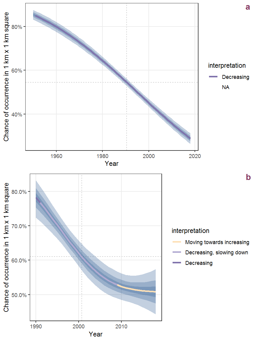
Figure R.14: The same as R.13, but the vertical axis is scaled to the range of the predicted values such that relative changes can be seen more easily. a: 1950 - 2018, b: 1990 - 2018.
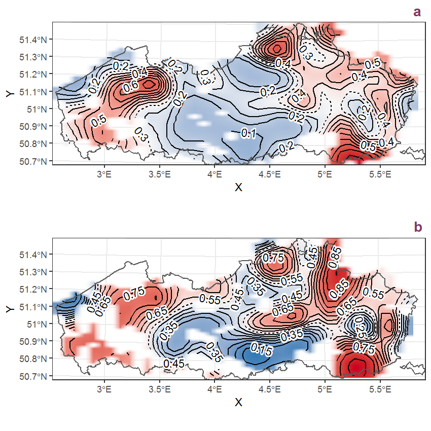
Figure R.15: Visualisation of the spatial smooth effect on the probability of Salix aurita L. presence in 1 km x 1 km squares where the species has been observed at least once. The probabilities (values on the contour lines) are conditional on the final year of observation and a list-length equal to 130. The dashed contour line demarcates zones where the species is expected to be more prevalent (red shades) from zones where the species is less prevalent (blue shades). a: 1950 - 2018, b: 1990 - 2018.
R.6 Salix caprea L.
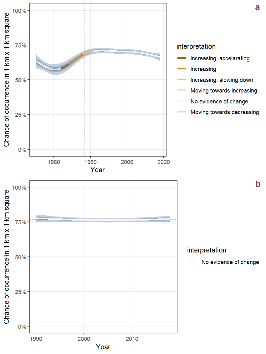
Figure R.16: Effect of year on the probability of Salix caprea L. presence in 1 km x 1 km squares where the species has been observed at least once. The fitted line shows the sum of the overall mean (the intercept), a conditional effect of list-length equal to 130 and the year-smoother. The vertical dashed lines indicate the year(s) where the year-smoother is zero. The 95% confidence band is shown in grey (including the variability around the intercept and the smoother). a: 1950 - 2018, b: 1990 - 2018.
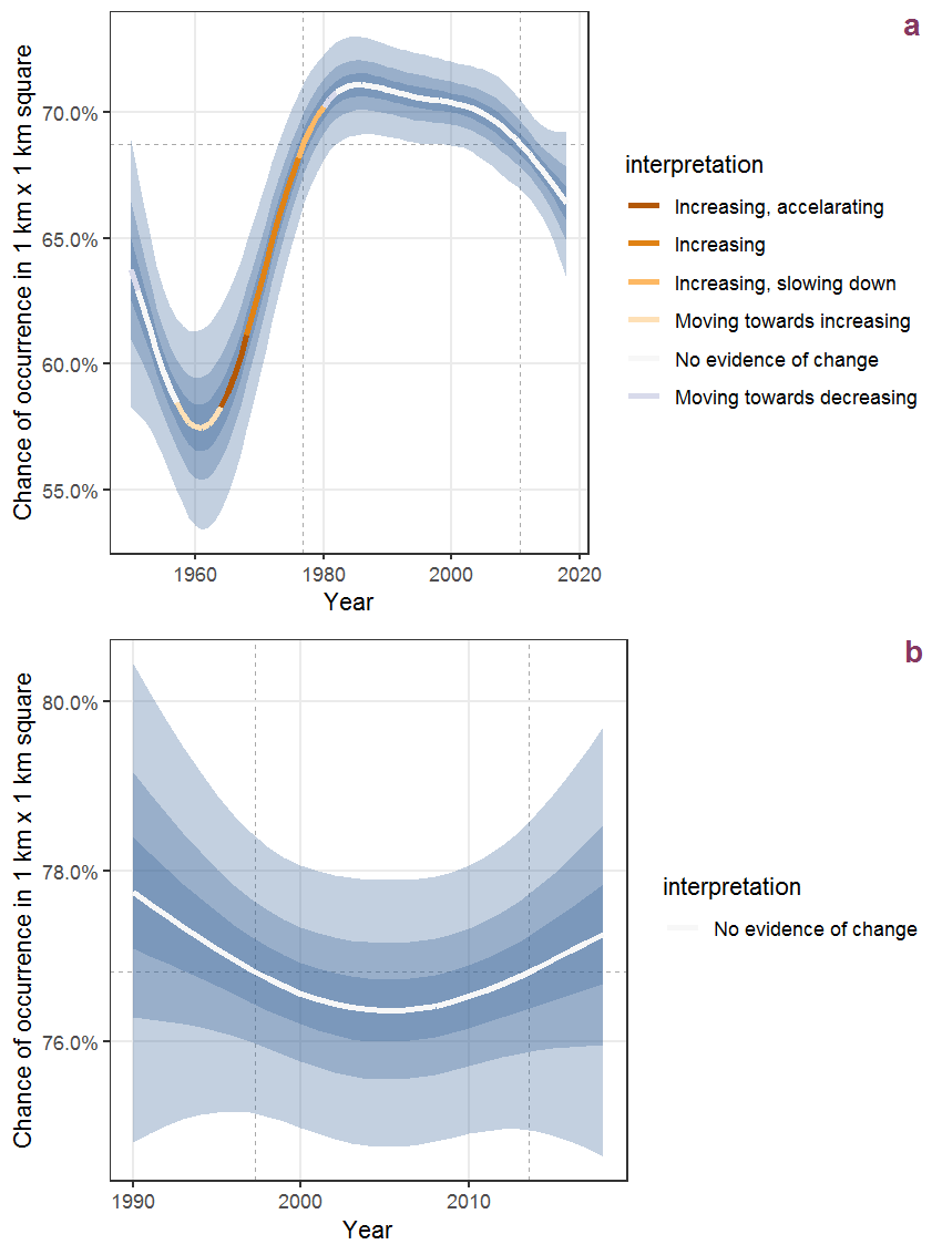
Figure R.17: The same as R.16, but the vertical axis is scaled to the range of the predicted values such that relative changes can be seen more easily. a: 1950 - 2018, b: 1990 - 2018.
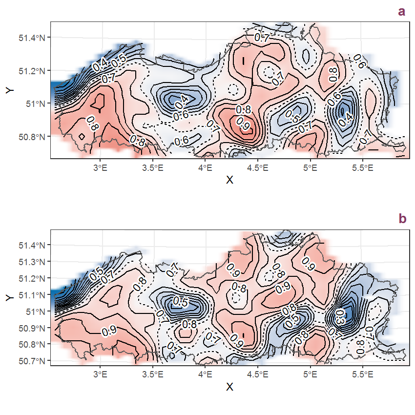
Figure R.18: Visualisation of the spatial smooth effect on the probability of Salix caprea L. presence in 1 km x 1 km squares where the species has been observed at least once. The probabilities (values on the contour lines) are conditional on the final year of observation and a list-length equal to 130. The dashed contour line demarcates zones where the species is expected to be more prevalent (red shades) from zones where the species is less prevalent (blue shades). a: 1950 - 2018, b: 1990 - 2018.
R.7 Salix fragilis L. (incl. kruisingen)
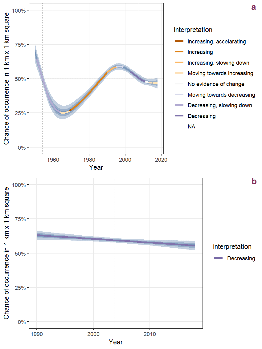
Figure R.19: Effect of year on the probability of Salix fragilis L. (incl. kruisingen) presence in 1 km x 1 km squares where the species has been observed at least once. The fitted line shows the sum of the overall mean (the intercept), a conditional effect of list-length equal to 130 and the year-smoother. The vertical dashed lines indicate the year(s) where the year-smoother is zero. The 95% confidence band is shown in grey (including the variability around the intercept and the smoother). a: 1950 - 2018, b: 1990 - 2018.
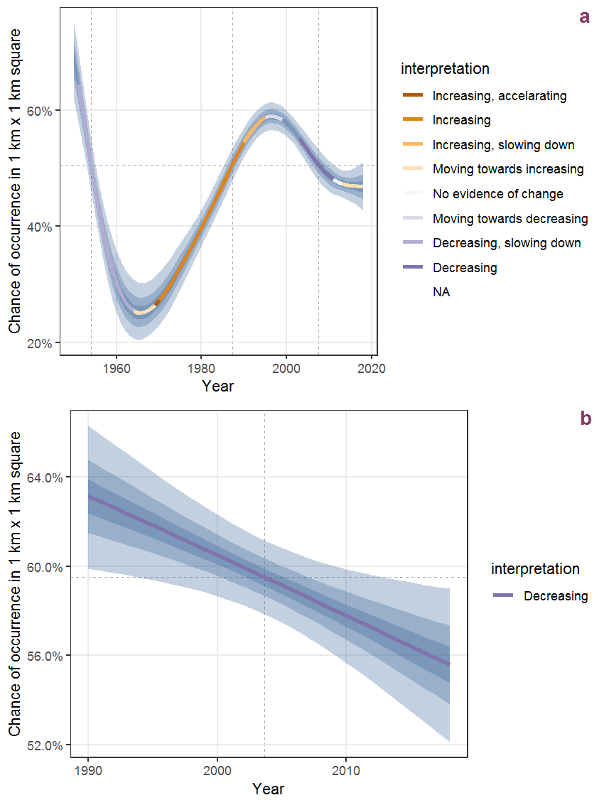
Figure R.20: The same as R.19, but the vertical axis is scaled to the range of the predicted values such that relative changes can be seen more easily. a: 1950 - 2018, b: 1990 - 2018.
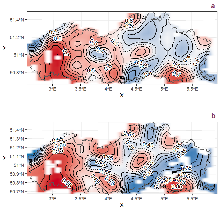
Figure R.21: Visualisation of the spatial smooth effect on the probability of Salix fragilis L. (incl. kruisingen) presence in 1 km x 1 km squares where the species has been observed at least once. The probabilities (values on the contour lines) are conditional on the final year of observation and a list-length equal to 130. The dashed contour line demarcates zones where the species is expected to be more prevalent (red shades) from zones where the species is less prevalent (blue shades). a: 1950 - 2018, b: 1990 - 2018.
R.8 Salix repens L.
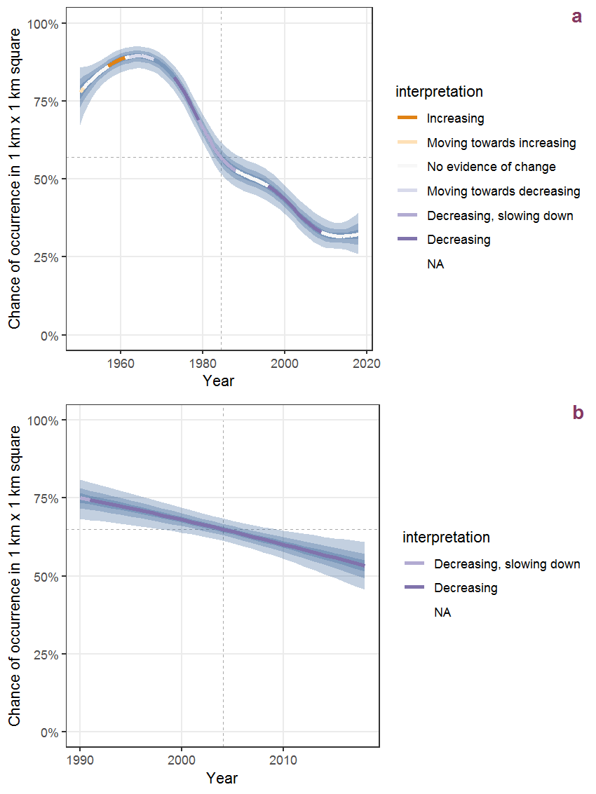
Figure R.22: Effect of year on the probability of Salix repens L. presence in 1 km x 1 km squares where the species has been observed at least once. The fitted line shows the sum of the overall mean (the intercept), a conditional effect of list-length equal to 130 and the year-smoother. The vertical dashed lines indicate the year(s) where the year-smoother is zero. The 95% confidence band is shown in grey (including the variability around the intercept and the smoother). a: 1950 - 2018, b: 1990 - 2018.
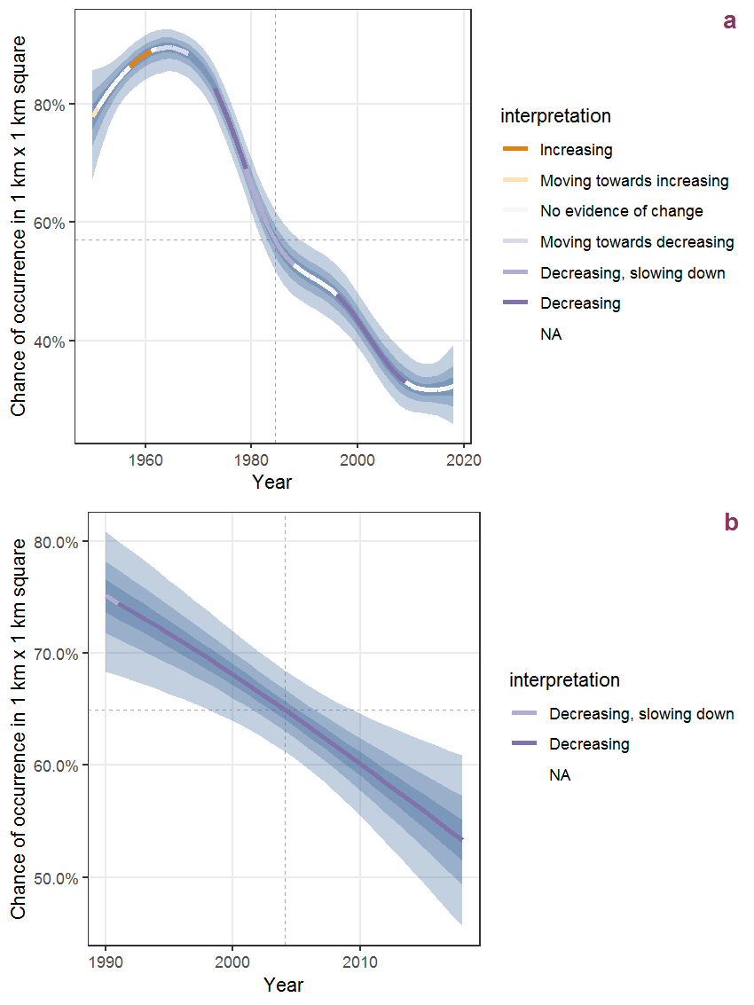
Figure R.23: The same as R.22, but the vertical axis is scaled to the range of the predicted values such that relative changes can be seen more easily. a: 1950 - 2018, b: 1990 - 2018.
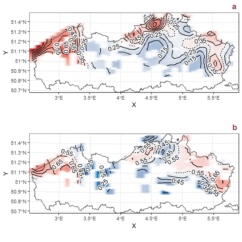
Figure R.24: Visualisation of the spatial smooth effect on the probability of Salix repens L. presence in 1 km x 1 km squares where the species has been observed at least once. The probabilities (values on the contour lines) are conditional on the final year of observation and a list-length equal to 130. The dashed contour line demarcates zones where the species is expected to be more prevalent (red shades) from zones where the species is less prevalent (blue shades). a: 1950 - 2018, b: 1990 - 2018.
R.9 Salix triandra L.
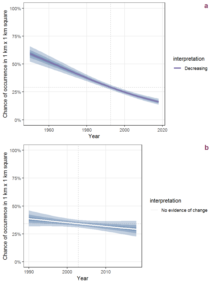
Figure R.25: Effect of year on the probability of Salix triandra L. presence in 1 km x 1 km squares where the species has been observed at least once. The fitted line shows the sum of the overall mean (the intercept), a conditional effect of list-length equal to 130 and the year-smoother. The vertical dashed lines indicate the year(s) where the year-smoother is zero. The 95% confidence band is shown in grey (including the variability around the intercept and the smoother). a: 1950 - 2018, b: 1990 - 2018.
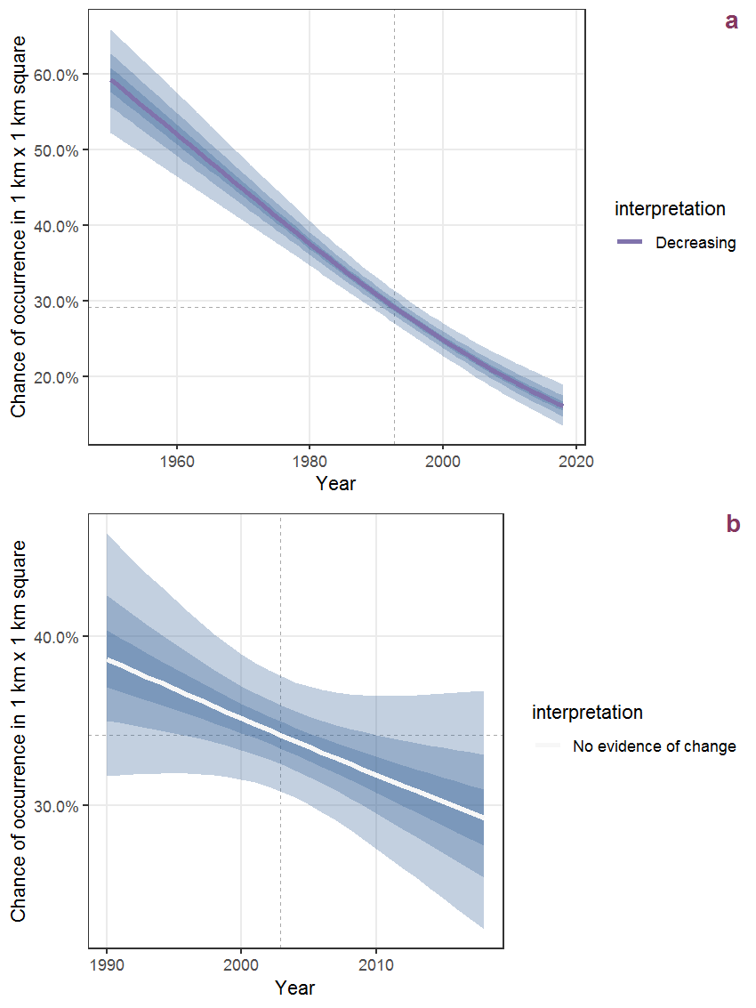
Figure R.26: The same as R.25, but the vertical axis is scaled to the range of the predicted values such that relative changes can be seen more easily. a: 1950 - 2018, b: 1990 - 2018.
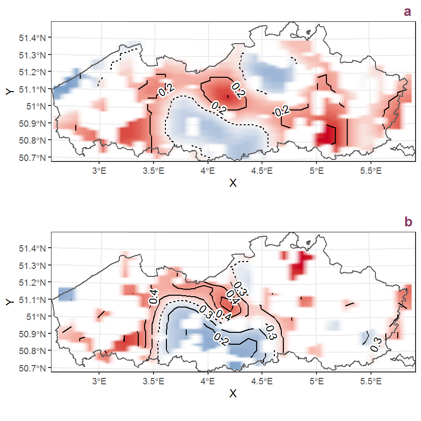
Figure R.27: Visualisation of the spatial smooth effect on the probability of Salix triandra L. presence in 1 km x 1 km squares where the species has been observed at least once. The probabilities (values on the contour lines) are conditional on the final year of observation and a list-length equal to 130. The dashed contour line demarcates zones where the species is expected to be more prevalent (red shades) from zones where the species is less prevalent (blue shades). a: 1950 - 2018, b: 1990 - 2018.
R.10 Salix viminalis L.
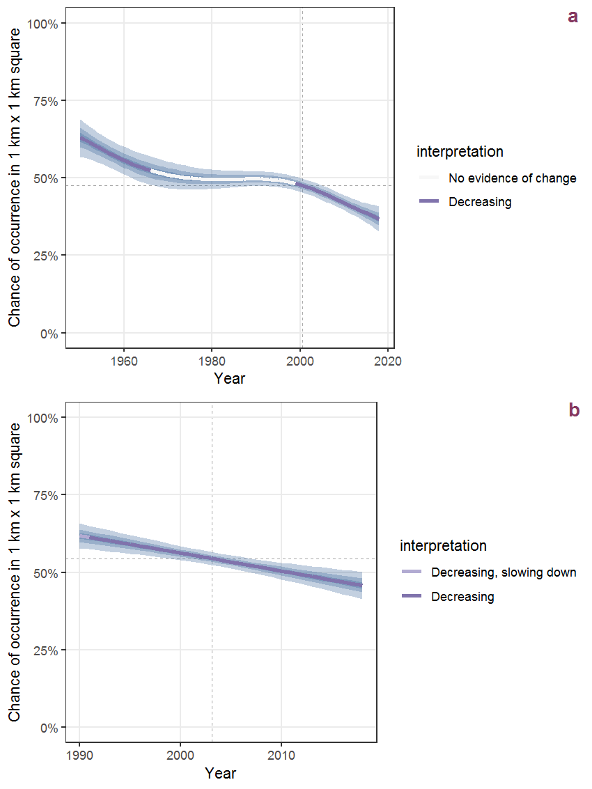
Figure R.28: Effect of year on the probability of Salix viminalis L. presence in 1 km x 1 km squares where the species has been observed at least once. The fitted line shows the sum of the overall mean (the intercept), a conditional effect of list-length equal to 130 and the year-smoother. The vertical dashed lines indicate the year(s) where the year-smoother is zero. The 95% confidence band is shown in grey (including the variability around the intercept and the smoother). a: 1950 - 2018, b: 1990 - 2018.
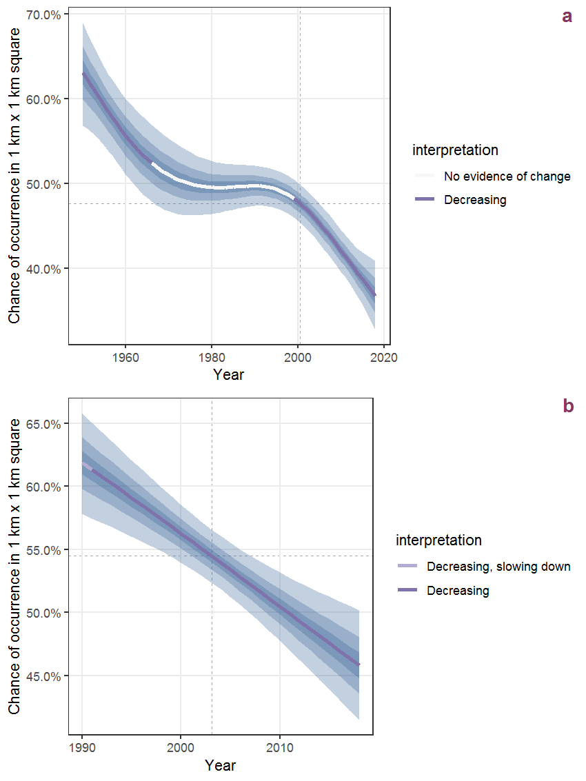
Figure R.29: The same as R.28, but the vertical axis is scaled to the range of the predicted values such that relative changes can be seen more easily. a: 1950 - 2018, b: 1990 - 2018.
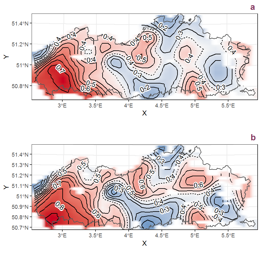
Figure R.30: Visualisation of the spatial smooth effect on the probability of Salix viminalis L. presence in 1 km x 1 km squares where the species has been observed at least once. The probabilities (values on the contour lines) are conditional on the final year of observation and a list-length equal to 130. The dashed contour line demarcates zones where the species is expected to be more prevalent (red shades) from zones where the species is less prevalent (blue shades). a: 1950 - 2018, b: 1990 - 2018.
R.11 Sambucus nigra L.
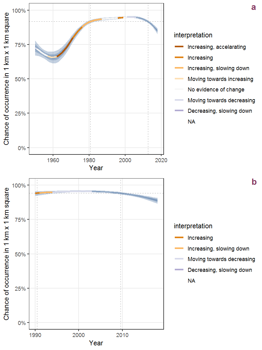
Figure R.31: Effect of year on the probability of Sambucus nigra L. presence in 1 km x 1 km squares where the species has been observed at least once. The fitted line shows the sum of the overall mean (the intercept), a conditional effect of list-length equal to 130 and the year-smoother. The vertical dashed lines indicate the year(s) where the year-smoother is zero. The 95% confidence band is shown in grey (including the variability around the intercept and the smoother). a: 1950 - 2018, b: 1990 - 2018.
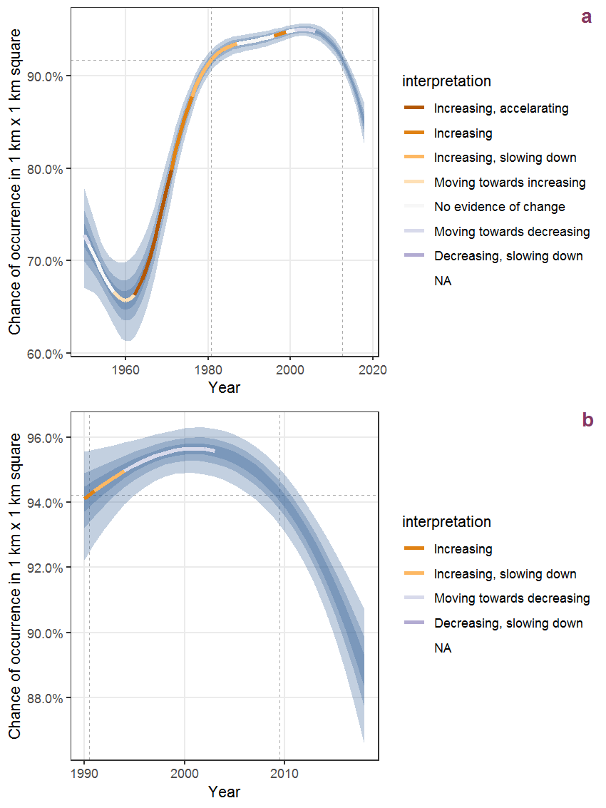
Figure R.32: The same as R.31, but the vertical axis is scaled to the range of the predicted values such that relative changes can be seen more easily. a: 1950 - 2018, b: 1990 - 2018.
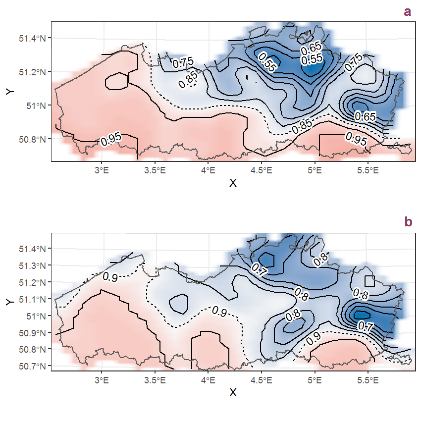
Figure R.33: Visualisation of the spatial smooth effect on the probability of Sambucus nigra L. presence in 1 km x 1 km squares where the species has been observed at least once. The probabilities (values on the contour lines) are conditional on the final year of observation and a list-length equal to 130. The dashed contour line demarcates zones where the species is expected to be more prevalent (red shades) from zones where the species is less prevalent (blue shades). a: 1950 - 2018, b: 1990 - 2018.
R.12 Saponaria officinalis L.
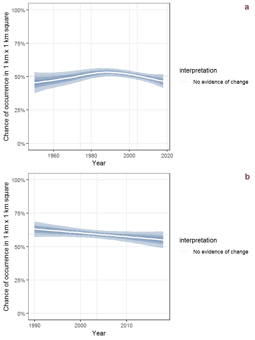
Figure R.34: Effect of year on the probability of Saponaria officinalis L. presence in 1 km x 1 km squares where the species has been observed at least once. The fitted line shows the sum of the overall mean (the intercept), a conditional effect of list-length equal to 130 and the year-smoother. The vertical dashed lines indicate the year(s) where the year-smoother is zero. The 95% confidence band is shown in grey (including the variability around the intercept and the smoother). a: 1950 - 2018, b: 1990 - 2018.
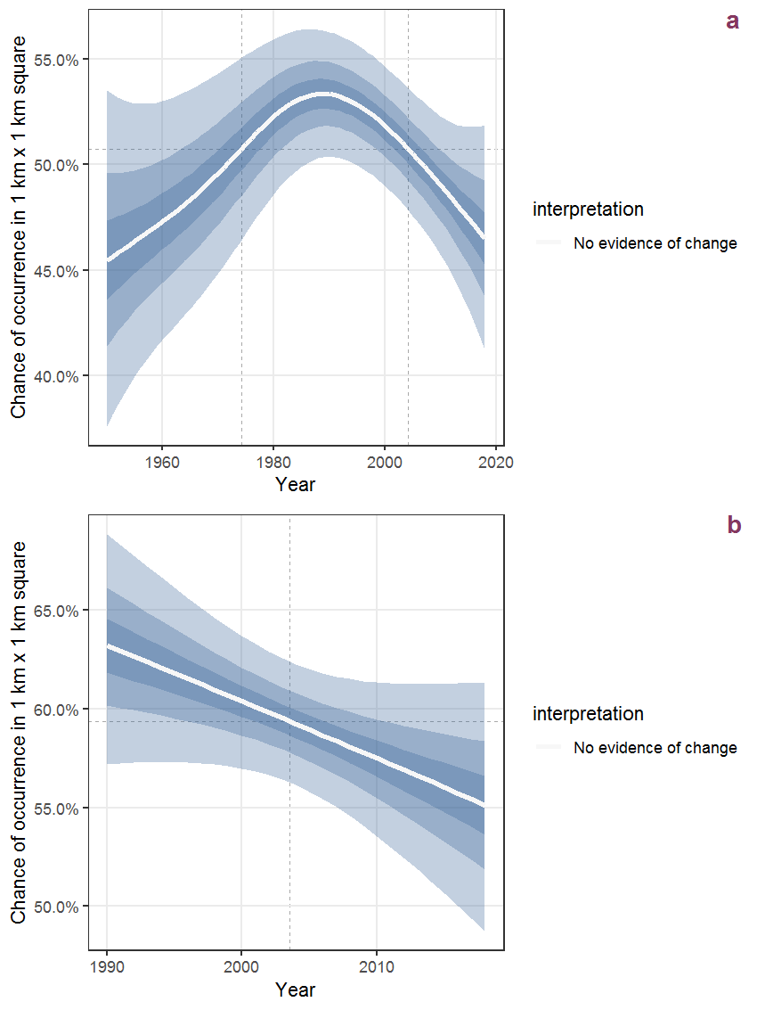
Figure R.35: The same as R.34, but the vertical axis is scaled to the range of the predicted values such that relative changes can be seen more easily. a: 1950 - 2018, b: 1990 - 2018.
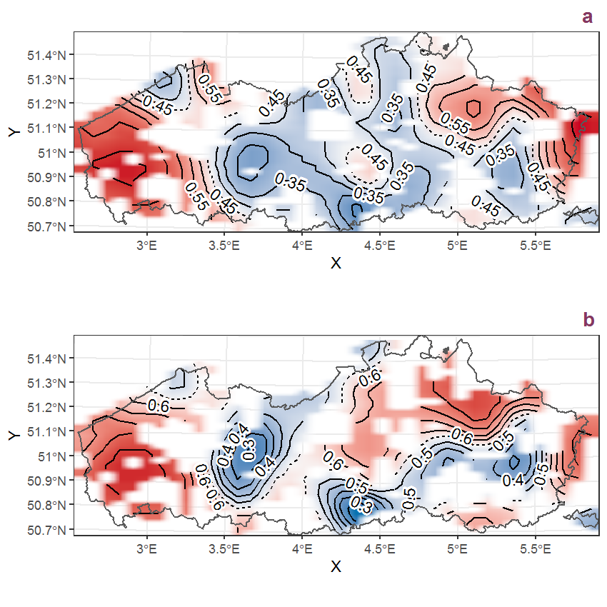
Figure R.36: Visualisation of the spatial smooth effect on the probability of Saponaria officinalis L. presence in 1 km x 1 km squares where the species has been observed at least once. The probabilities (values on the contour lines) are conditional on the final year of observation and a list-length equal to 130. The dashed contour line demarcates zones where the species is expected to be more prevalent (red shades) from zones where the species is less prevalent (blue shades). a: 1950 - 2018, b: 1990 - 2018.
R.13 Saxifraga granulata L.
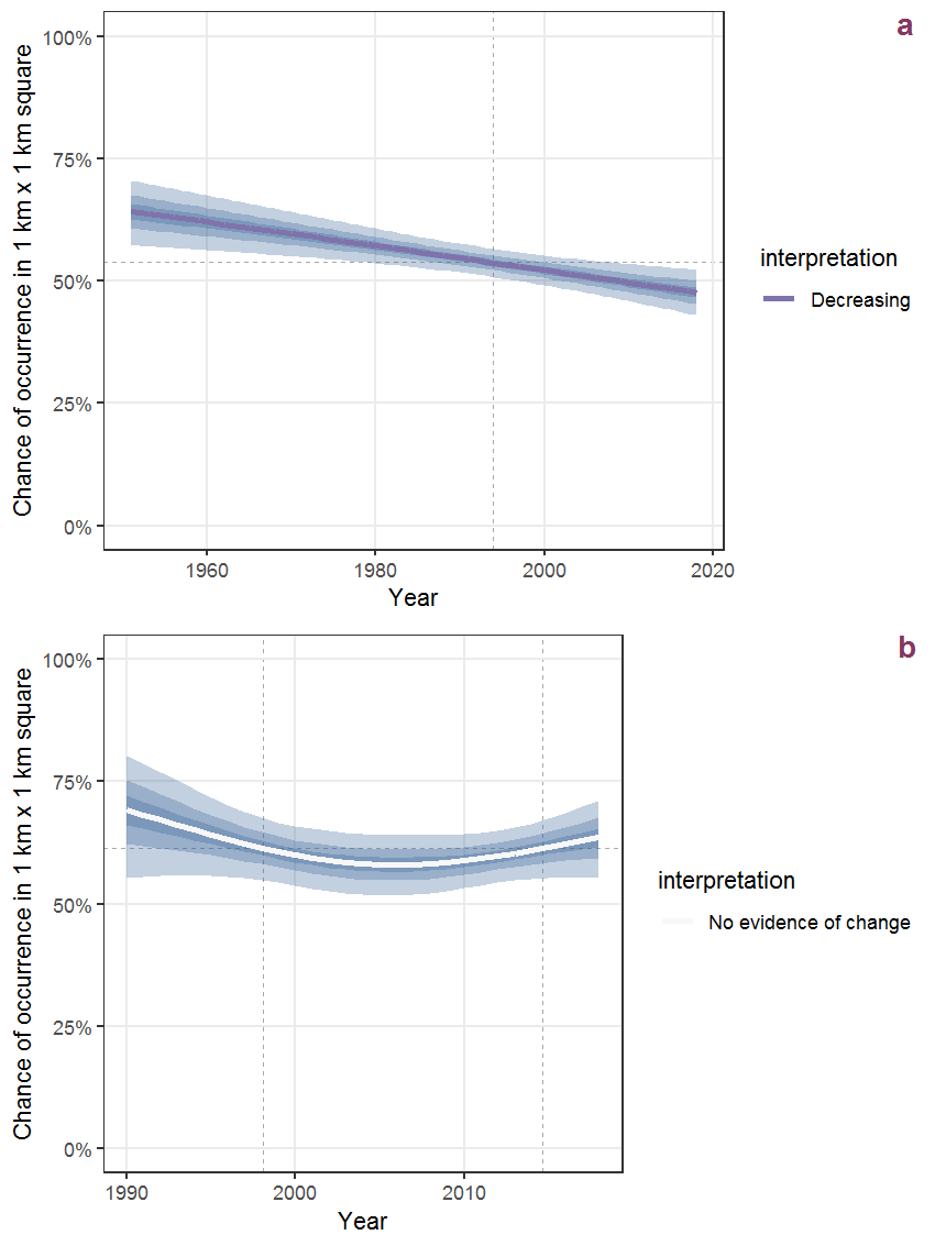
Figure R.37: Effect of year on the probability of Saxifraga granulata L. presence in 1 km x 1 km squares where the species has been observed at least once. The fitted line shows the sum of the overall mean (the intercept), a conditional effect of list-length equal to 130 and the year-smoother. The vertical dashed lines indicate the year(s) where the year-smoother is zero. The 95% confidence band is shown in grey (including the variability around the intercept and the smoother). a: 1950 - 2018, b: 1990 - 2018.
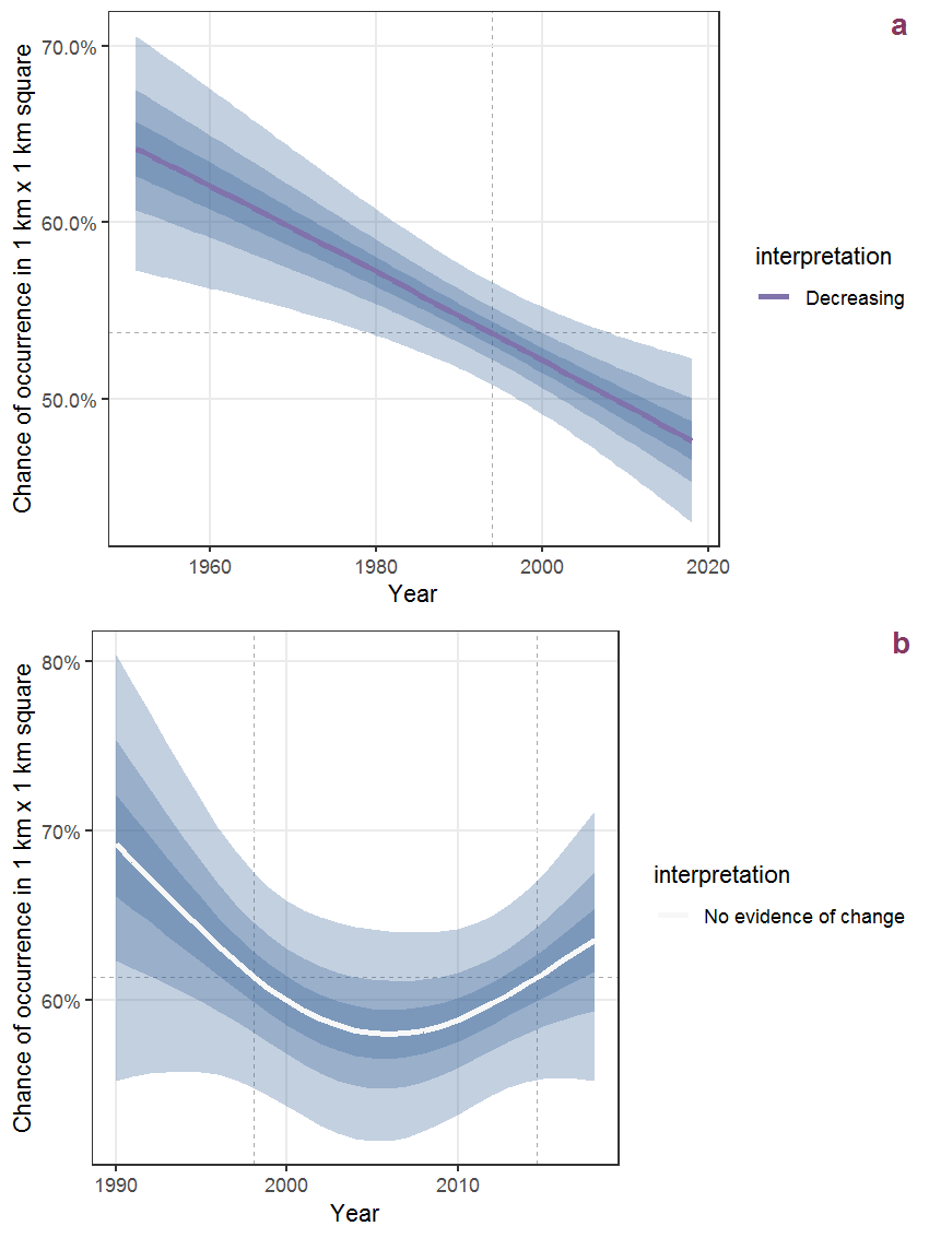
Figure R.38: The same as R.37, but the vertical axis is scaled to the range of the predicted values such that relative changes can be seen more easily. a: 1950 - 2018, b: 1990 - 2018.
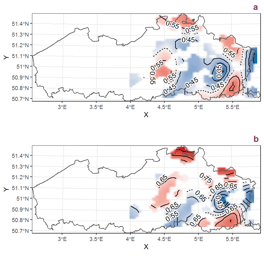
Figure R.39: Visualisation of the spatial smooth effect on the probability of Saxifraga granulata L. presence in 1 km x 1 km squares where the species has been observed at least once. The probabilities (values on the contour lines) are conditional on the final year of observation and a list-length equal to 130. The dashed contour line demarcates zones where the species is expected to be more prevalent (red shades) from zones where the species is less prevalent (blue shades). a: 1950 - 2018, b: 1990 - 2018.
R.14 Saxifraga tridactylites L.
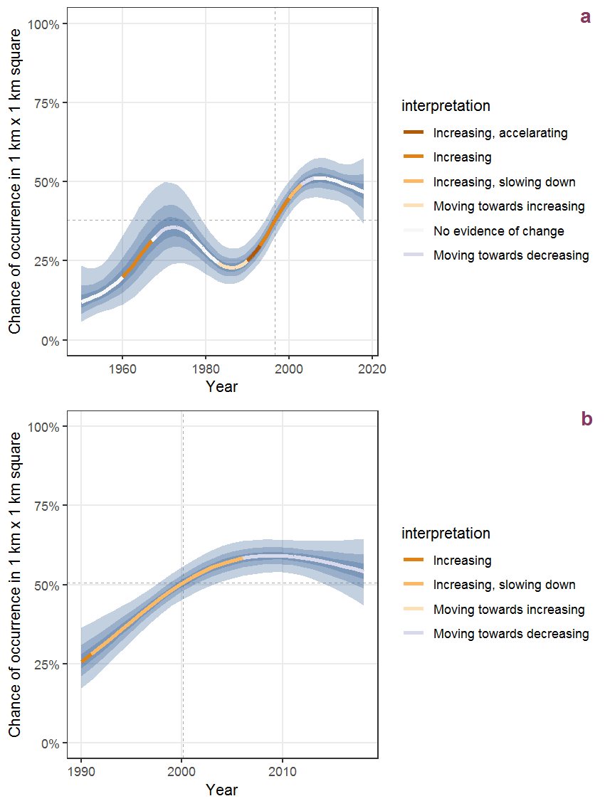
Figure R.40: Effect of year on the probability of Saxifraga tridactylites L. presence in 1 km x 1 km squares where the species has been observed at least once. The fitted line shows the sum of the overall mean (the intercept), a conditional effect of list-length equal to 130 and the year-smoother. The vertical dashed lines indicate the year(s) where the year-smoother is zero. The 95% confidence band is shown in grey (including the variability around the intercept and the smoother). a: 1950 - 2018, b: 1990 - 2018.
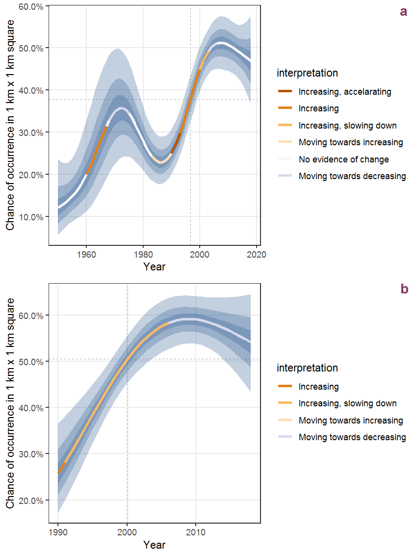
Figure R.41: The same as R.40, but the vertical axis is scaled to the range of the predicted values such that relative changes can be seen more easily. a: 1950 - 2018, b: 1990 - 2018.
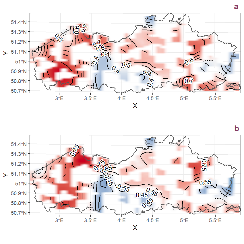
Figure R.42: Visualisation of the spatial smooth effect on the probability of Saxifraga tridactylites L. presence in 1 km x 1 km squares where the species has been observed at least once. The probabilities (values on the contour lines) are conditional on the final year of observation and a list-length equal to 130. The dashed contour line demarcates zones where the species is expected to be more prevalent (red shades) from zones where the species is less prevalent (blue shades). a: 1950 - 2018, b: 1990 - 2018.
R.15 Hyacinthoides hispanica (Mill.) Rothm.
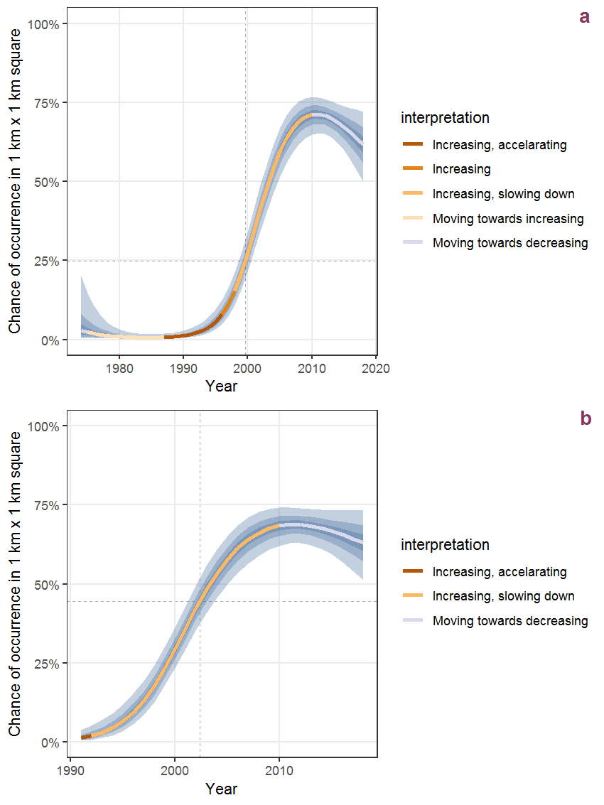
Figure R.43: Effect of year on the probability of Hyacinthoides hispanica (Mill.) Rothm. presence in 1 km x 1 km squares where the species has been observed at least once. The fitted line shows the sum of the overall mean (the intercept), a conditional effect of list-length equal to 130 and the year-smoother. The vertical dashed lines indicate the year(s) where the year-smoother is zero. The 95% confidence band is shown in grey (including the variability around the intercept and the smoother). a: 1950 - 2018, b: 1990 - 2018.
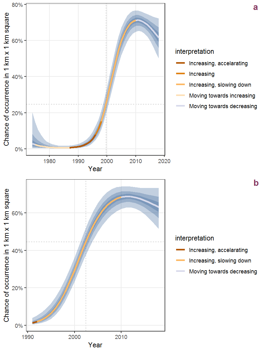
Figure R.44: The same as R.43, but the vertical axis is scaled to the range of the predicted values such that relative changes can be seen more easily. a: 1950 - 2018, b: 1990 - 2018.
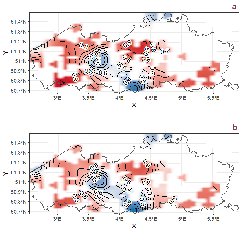
Figure R.45: Visualisation of the spatial smooth effect on the probability of Hyacinthoides hispanica (Mill.) Rothm. presence in 1 km x 1 km squares where the species has been observed at least once. The probabilities (values on the contour lines) are conditional on the final year of observation and a list-length equal to 130. The dashed contour line demarcates zones where the species is expected to be more prevalent (red shades) from zones where the species is less prevalent (blue shades). a: 1950 - 2018, b: 1990 - 2018.
R.16 Hyacinthoides non-scripta (L.) Chouard ex Rothm.
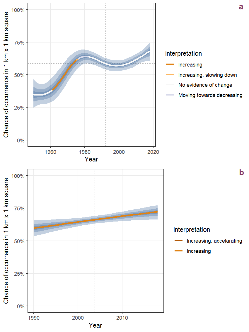
Figure R.46: Effect of year on the probability of Hyacinthoides non-scripta (L.) Chouard ex Rothm. presence in 1 km x 1 km squares where the species has been observed at least once. The fitted line shows the sum of the overall mean (the intercept), a conditional effect of list-length equal to 130 and the year-smoother. The vertical dashed lines indicate the year(s) where the year-smoother is zero. The 95% confidence band is shown in grey (including the variability around the intercept and the smoother). a: 1950 - 2018, b: 1990 - 2018.
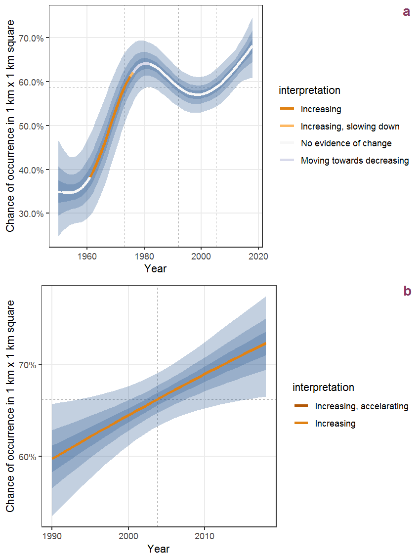
Figure R.47: The same as R.46, but the vertical axis is scaled to the range of the predicted values such that relative changes can be seen more easily. a: 1950 - 2018, b: 1990 - 2018.
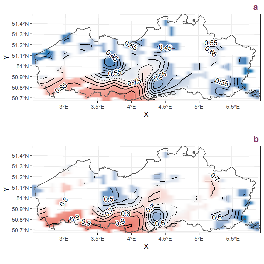
Figure R.48: Visualisation of the spatial smooth effect on the probability of Hyacinthoides non-scripta (L.) Chouard ex Rothm. presence in 1 km x 1 km squares where the species has been observed at least once. The probabilities (values on the contour lines) are conditional on the final year of observation and a list-length equal to 130. The dashed contour line demarcates zones where the species is expected to be more prevalent (red shades) from zones where the species is less prevalent (blue shades). a: 1950 - 2018, b: 1990 - 2018.
R.17 Scirpus maritimus L.
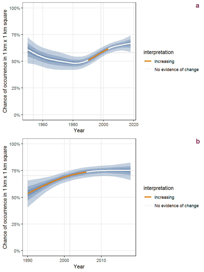
Figure R.49: Effect of year on the probability of Scirpus maritimus L. presence in 1 km x 1 km squares where the species has been observed at least once. The fitted line shows the sum of the overall mean (the intercept), a conditional effect of list-length equal to 130 and the year-smoother. The vertical dashed lines indicate the year(s) where the year-smoother is zero. The 95% confidence band is shown in grey (including the variability around the intercept and the smoother). a: 1950 - 2018, b: 1990 - 2018.
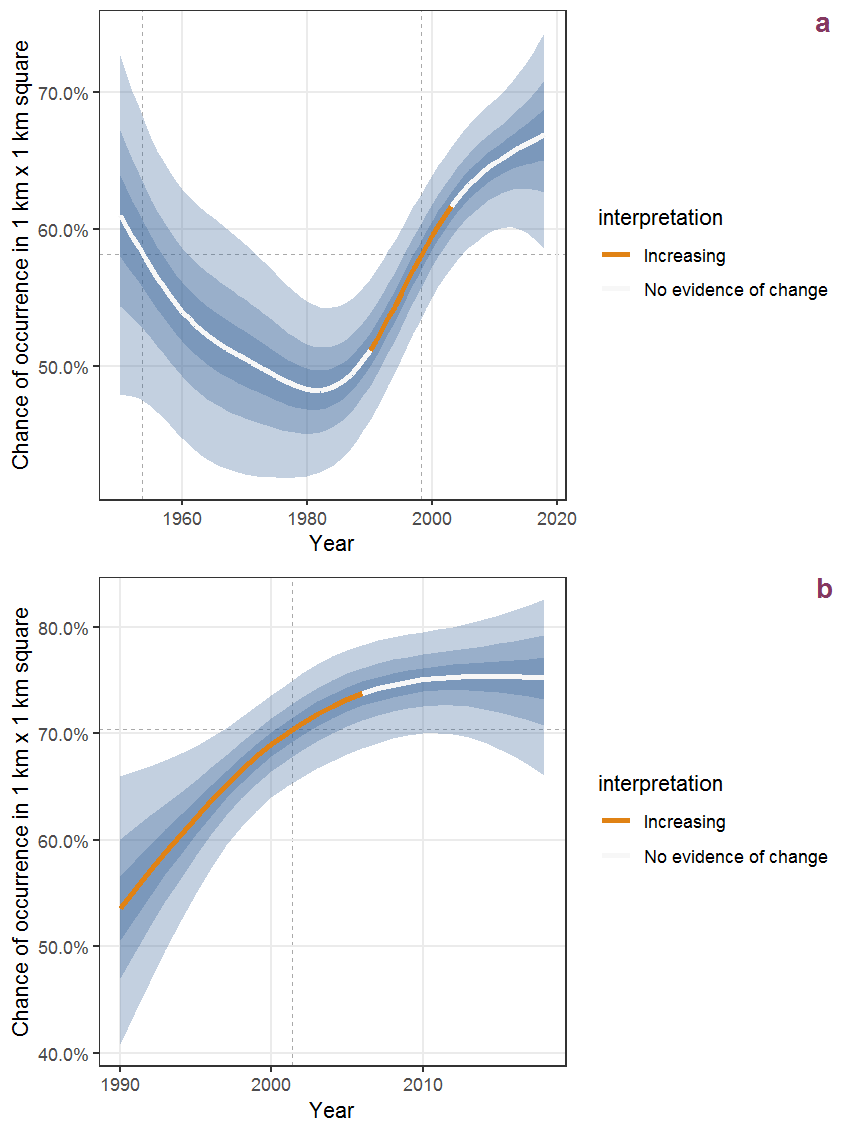
Figure R.50: The same as R.49, but the vertical axis is scaled to the range of the predicted values such that relative changes can be seen more easily. a: 1950 - 2018, b: 1990 - 2018.
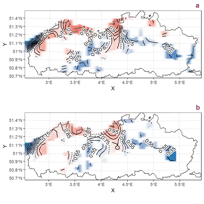
Figure R.51: Visualisation of the spatial smooth effect on the probability of Scirpus maritimus L. presence in 1 km x 1 km squares where the species has been observed at least once. The probabilities (values on the contour lines) are conditional on the final year of observation and a list-length equal to 130. The dashed contour line demarcates zones where the species is expected to be more prevalent (red shades) from zones where the species is less prevalent (blue shades). a: 1950 - 2018, b: 1990 - 2018.
R.18 Scirpus setaceus L.
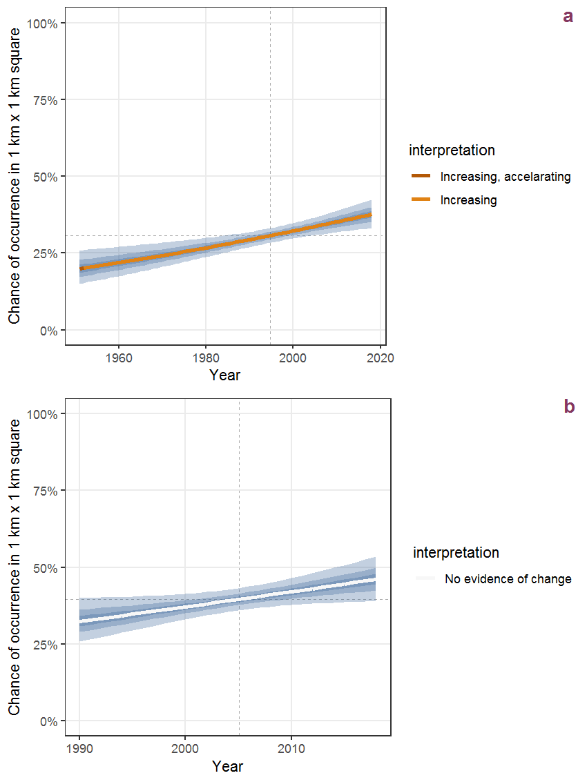
Figure R.52: Effect of year on the probability of Scirpus setaceus L. presence in 1 km x 1 km squares where the species has been observed at least once. The fitted line shows the sum of the overall mean (the intercept), a conditional effect of list-length equal to 130 and the year-smoother. The vertical dashed lines indicate the year(s) where the year-smoother is zero. The 95% confidence band is shown in grey (including the variability around the intercept and the smoother). a: 1950 - 2018, b: 1990 - 2018.
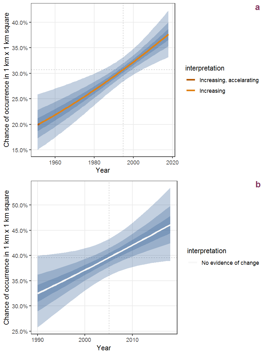
Figure R.53: The same as R.52, but the vertical axis is scaled to the range of the predicted values such that relative changes can be seen more easily. a: 1950 - 2018, b: 1990 - 2018.
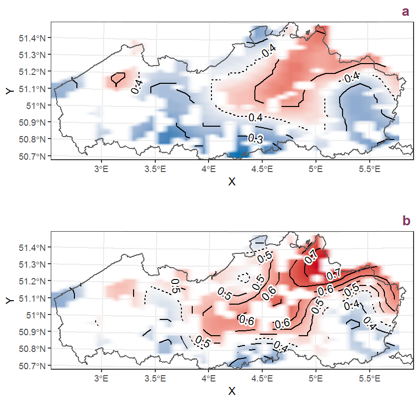
Figure R.54: Visualisation of the spatial smooth effect on the probability of Scirpus setaceus L. presence in 1 km x 1 km squares where the species has been observed at least once. The probabilities (values on the contour lines) are conditional on the final year of observation and a list-length equal to 130. The dashed contour line demarcates zones where the species is expected to be more prevalent (red shades) from zones where the species is less prevalent (blue shades). a: 1950 - 2018, b: 1990 - 2018.
R.19 Scirpus sylvaticus L.
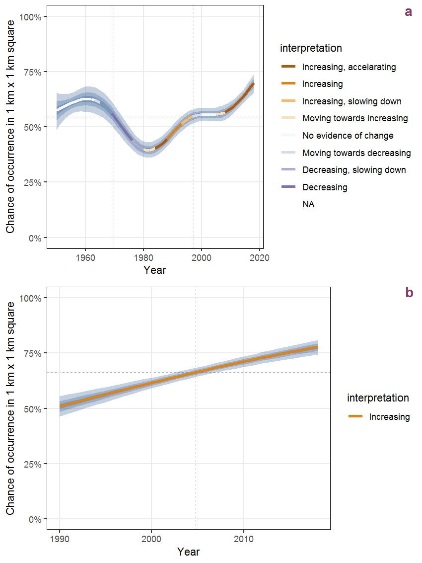
Figure R.55: Effect of year on the probability of Scirpus sylvaticus L. presence in 1 km x 1 km squares where the species has been observed at least once. The fitted line shows the sum of the overall mean (the intercept), a conditional effect of list-length equal to 130 and the year-smoother. The vertical dashed lines indicate the year(s) where the year-smoother is zero. The 95% confidence band is shown in grey (including the variability around the intercept and the smoother). a: 1950 - 2018, b: 1990 - 2018.
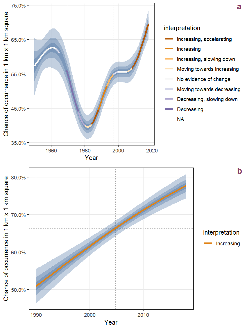
Figure R.56: The same as R.55, but the vertical axis is scaled to the range of the predicted values such that relative changes can be seen more easily. a: 1950 - 2018, b: 1990 - 2018.
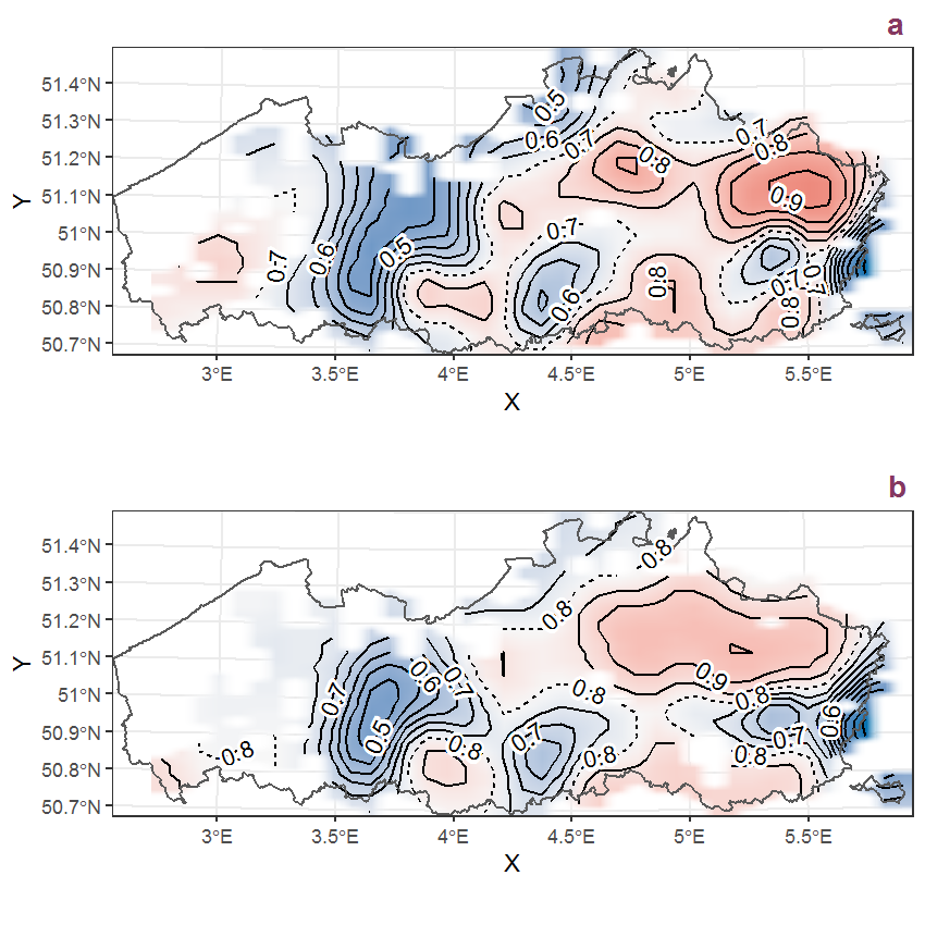
Figure R.57: Visualisation of the spatial smooth effect on the probability of Scirpus sylvaticus L. presence in 1 km x 1 km squares where the species has been observed at least once. The probabilities (values on the contour lines) are conditional on the final year of observation and a list-length equal to 130. The dashed contour line demarcates zones where the species is expected to be more prevalent (red shades) from zones where the species is less prevalent (blue shades). a: 1950 - 2018, b: 1990 - 2018.
R.20 Scleranthus annuus L.
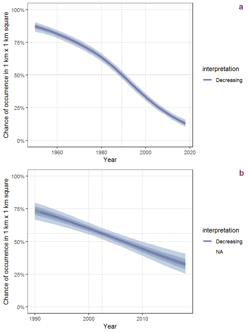
Figure R.58: Effect of year on the probability of Scleranthus annuus L. presence in 1 km x 1 km squares where the species has been observed at least once. The fitted line shows the sum of the overall mean (the intercept), a conditional effect of list-length equal to 130 and the year-smoother. The vertical dashed lines indicate the year(s) where the year-smoother is zero. The 95% confidence band is shown in grey (including the variability around the intercept and the smoother). a: 1950 - 2018, b: 1990 - 2018.
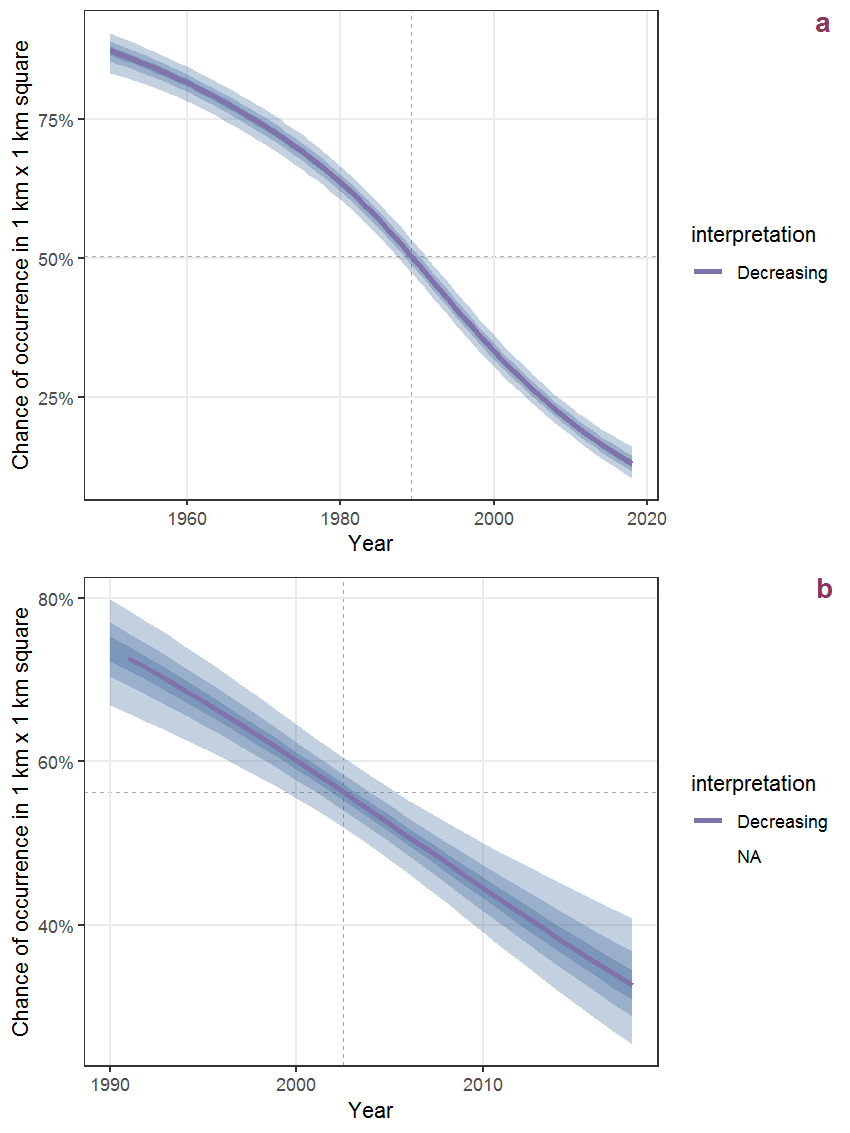
Figure R.59: The same as R.58, but the vertical axis is scaled to the range of the predicted values such that relative changes can be seen more easily. a: 1950 - 2018, b: 1990 - 2018.
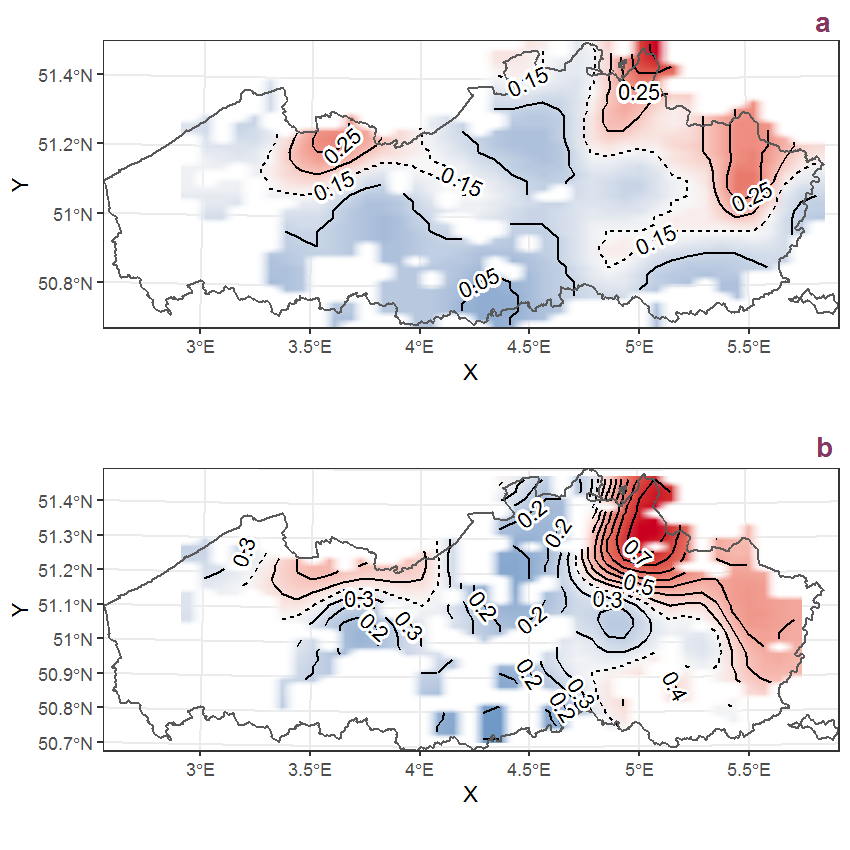
Figure R.60: Visualisation of the spatial smooth effect on the probability of Scleranthus annuus L. presence in 1 km x 1 km squares where the species has been observed at least once. The probabilities (values on the contour lines) are conditional on the final year of observation and a list-length equal to 130. The dashed contour line demarcates zones where the species is expected to be more prevalent (red shades) from zones where the species is less prevalent (blue shades). a: 1950 - 2018, b: 1990 - 2018.
R.21 Scrophularia auriculata L.
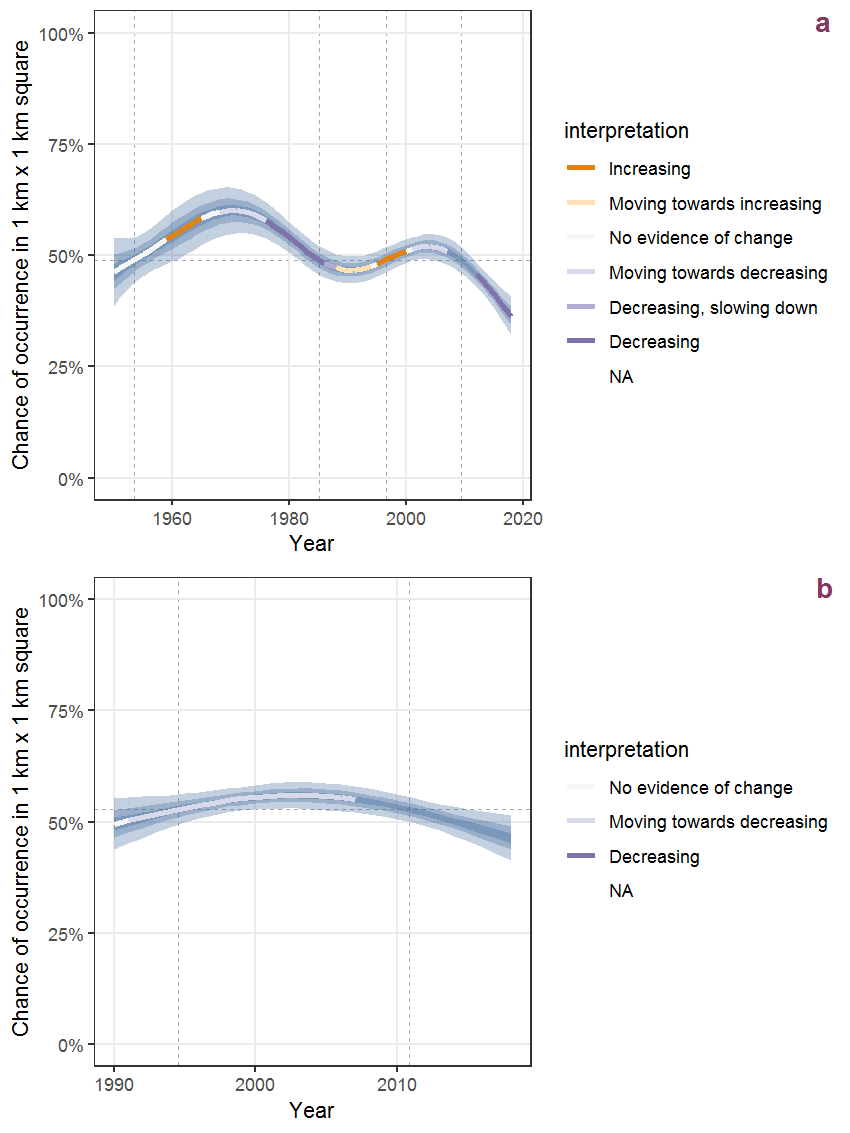
Figure R.61: Effect of year on the probability of Scrophularia auriculata L. presence in 1 km x 1 km squares where the species has been observed at least once. The fitted line shows the sum of the overall mean (the intercept), a conditional effect of list-length equal to 130 and the year-smoother. The vertical dashed lines indicate the year(s) where the year-smoother is zero. The 95% confidence band is shown in grey (including the variability around the intercept and the smoother). a: 1950 - 2018, b: 1990 - 2018.
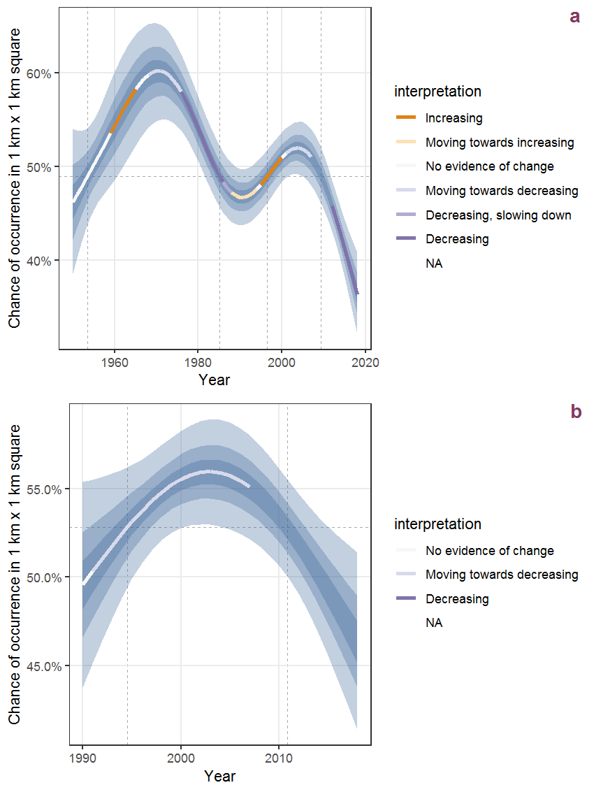
Figure R.62: The same as R.61, but the vertical axis is scaled to the range of the predicted values such that relative changes can be seen more easily. a: 1950 - 2018, b: 1990 - 2018.
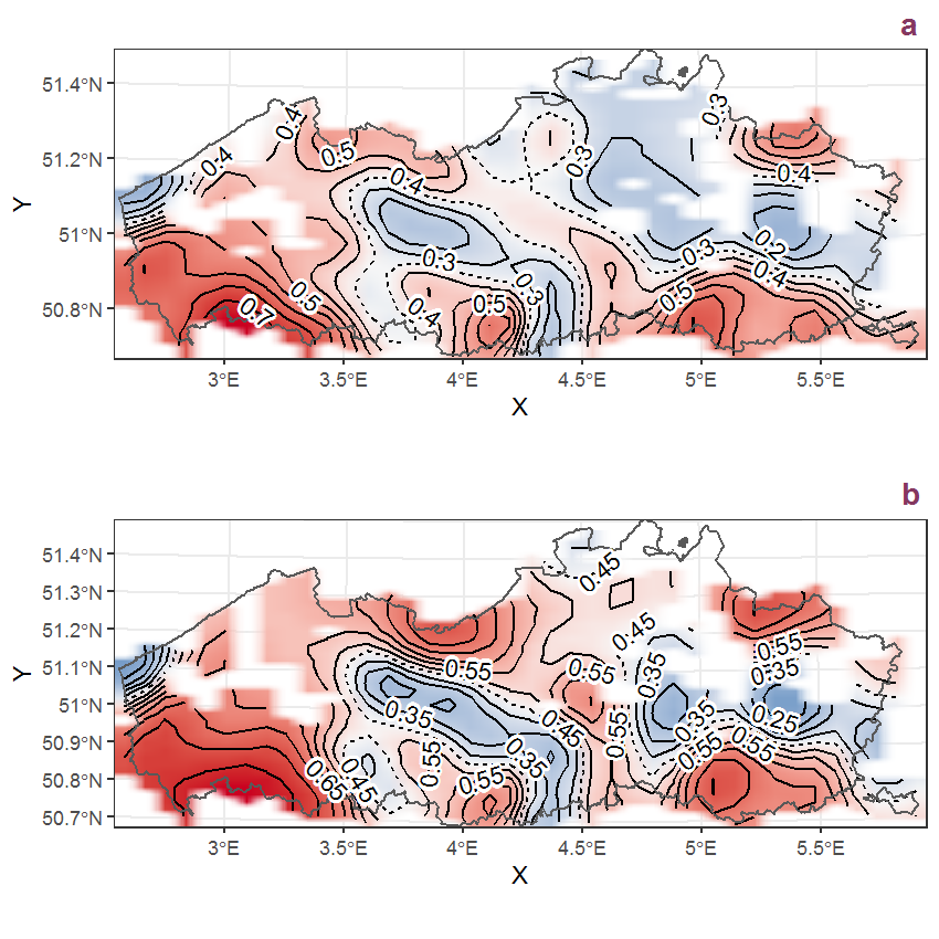
Figure R.63: Visualisation of the spatial smooth effect on the probability of Scrophularia auriculata L. presence in 1 km x 1 km squares where the species has been observed at least once. The probabilities (values on the contour lines) are conditional on the final year of observation and a list-length equal to 130. The dashed contour line demarcates zones where the species is expected to be more prevalent (red shades) from zones where the species is less prevalent (blue shades). a: 1950 - 2018, b: 1990 - 2018.
R.22 Scrophularia nodosa L.
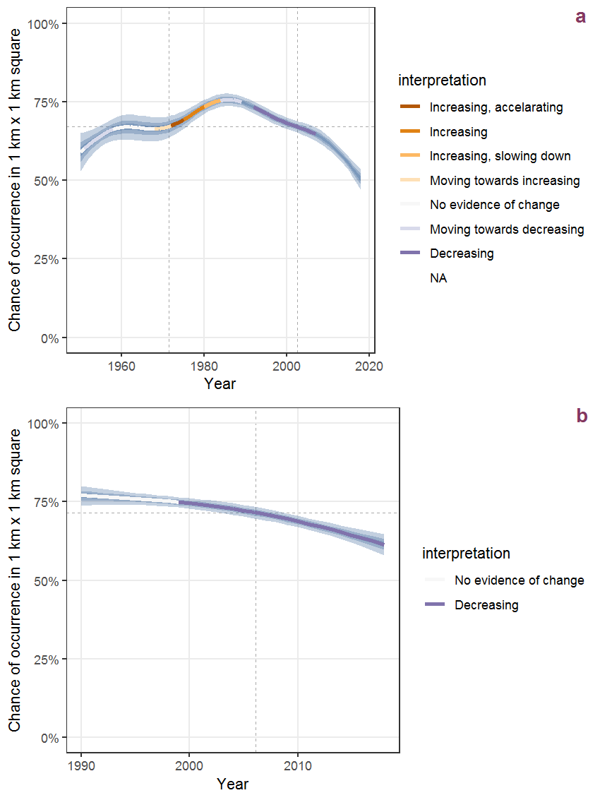
Figure R.64: Effect of year on the probability of Scrophularia nodosa L. presence in 1 km x 1 km squares where the species has been observed at least once. The fitted line shows the sum of the overall mean (the intercept), a conditional effect of list-length equal to 130 and the year-smoother. The vertical dashed lines indicate the year(s) where the year-smoother is zero. The 95% confidence band is shown in grey (including the variability around the intercept and the smoother). a: 1950 - 2018, b: 1990 - 2018.
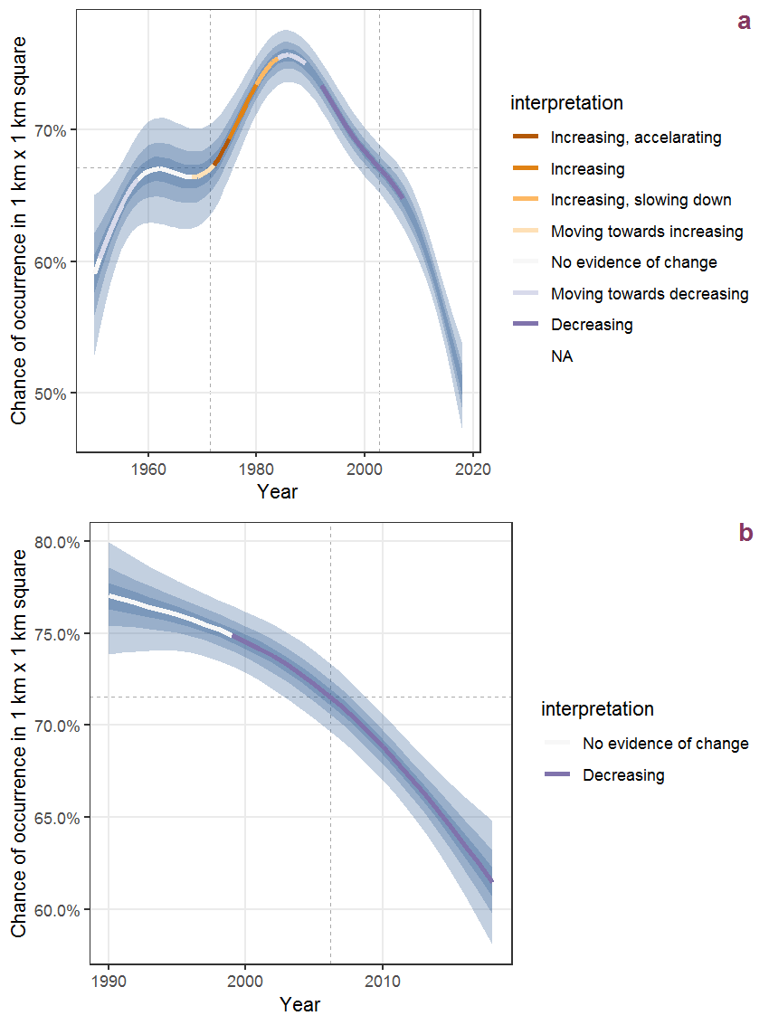
Figure R.65: The same as R.64, but the vertical axis is scaled to the range of the predicted values such that relative changes can be seen more easily. a: 1950 - 2018, b: 1990 - 2018.
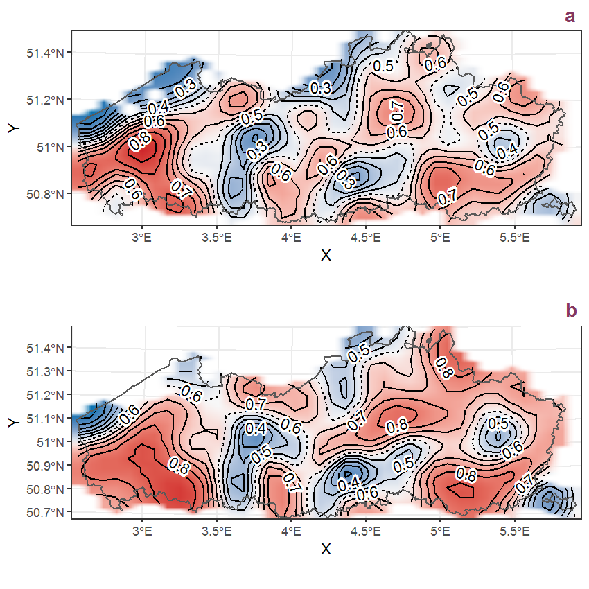
Figure R.66: Visualisation of the spatial smooth effect on the probability of Scrophularia nodosa L. presence in 1 km x 1 km squares where the species has been observed at least once. The probabilities (values on the contour lines) are conditional on the final year of observation and a list-length equal to 130. The dashed contour line demarcates zones where the species is expected to be more prevalent (red shades) from zones where the species is less prevalent (blue shades). a: 1950 - 2018, b: 1990 - 2018.
R.23 Scrophularia umbrosa Dum.
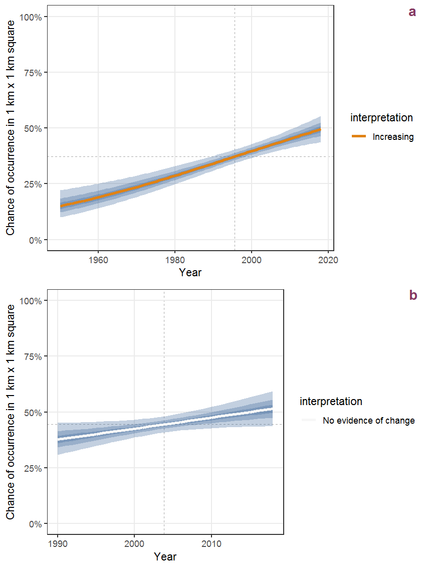
Figure R.67: Effect of year on the probability of Scrophularia umbrosa Dum. presence in 1 km x 1 km squares where the species has been observed at least once. The fitted line shows the sum of the overall mean (the intercept), a conditional effect of list-length equal to 130 and the year-smoother. The vertical dashed lines indicate the year(s) where the year-smoother is zero. The 95% confidence band is shown in grey (including the variability around the intercept and the smoother). a: 1950 - 2018, b: 1990 - 2018.
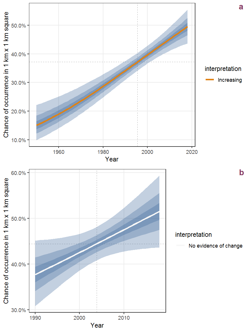
Figure R.68: The same as R.67, but the vertical axis is scaled to the range of the predicted values such that relative changes can be seen more easily. a: 1950 - 2018, b: 1990 - 2018.
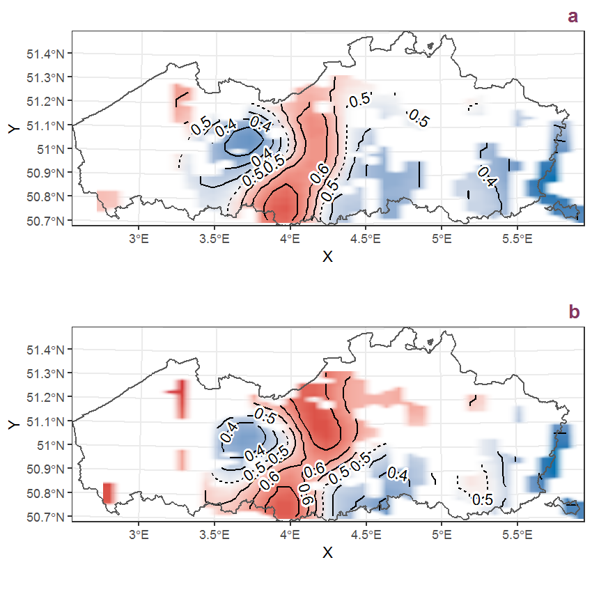
Figure R.69: Visualisation of the spatial smooth effect on the probability of Scrophularia umbrosa Dum. presence in 1 km x 1 km squares where the species has been observed at least once. The probabilities (values on the contour lines) are conditional on the final year of observation and a list-length equal to 130. The dashed contour line demarcates zones where the species is expected to be more prevalent (red shades) from zones where the species is less prevalent (blue shades). a: 1950 - 2018, b: 1990 - 2018.
R.24 Scutellaria galericulata L.
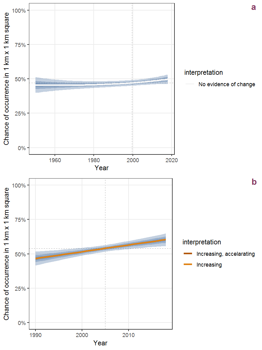
Figure R.70: Effect of year on the probability of Scutellaria galericulata L. presence in 1 km x 1 km squares where the species has been observed at least once. The fitted line shows the sum of the overall mean (the intercept), a conditional effect of list-length equal to 130 and the year-smoother. The vertical dashed lines indicate the year(s) where the year-smoother is zero. The 95% confidence band is shown in grey (including the variability around the intercept and the smoother). a: 1950 - 2018, b: 1990 - 2018.
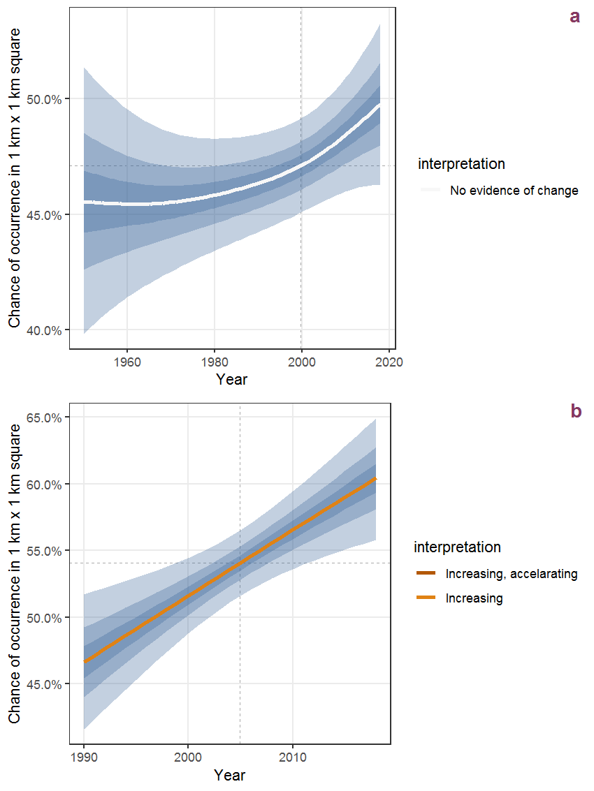
Figure R.71: The same as R.70, but the vertical axis is scaled to the range of the predicted values such that relative changes can be seen more easily. a: 1950 - 2018, b: 1990 - 2018.
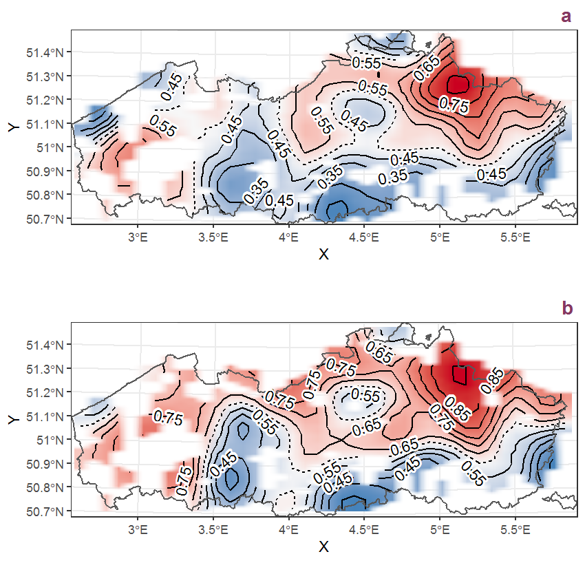
Figure R.72: Visualisation of the spatial smooth effect on the probability of Scutellaria galericulata L. presence in 1 km x 1 km squares where the species has been observed at least once. The probabilities (values on the contour lines) are conditional on the final year of observation and a list-length equal to 130. The dashed contour line demarcates zones where the species is expected to be more prevalent (red shades) from zones where the species is less prevalent (blue shades). a: 1950 - 2018, b: 1990 - 2018.
R.25 Sedum acre L.
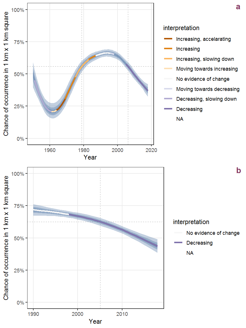
Figure R.73: Effect of year on the probability of Sedum acre L. presence in 1 km x 1 km squares where the species has been observed at least once. The fitted line shows the sum of the overall mean (the intercept), a conditional effect of list-length equal to 130 and the year-smoother. The vertical dashed lines indicate the year(s) where the year-smoother is zero. The 95% confidence band is shown in grey (including the variability around the intercept and the smoother). a: 1950 - 2018, b: 1990 - 2018.
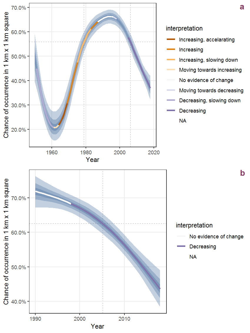
Figure R.74: The same as R.73, but the vertical axis is scaled to the range of the predicted values such that relative changes can be seen more easily. a: 1950 - 2018, b: 1990 - 2018.
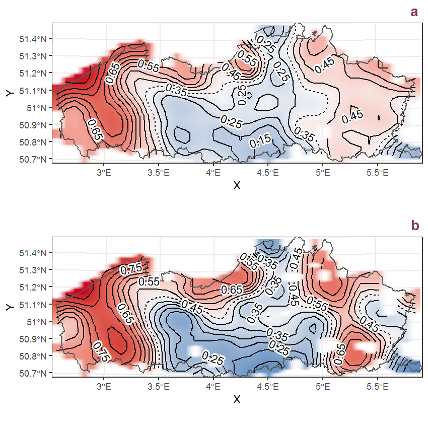
Figure R.75: Visualisation of the spatial smooth effect on the probability of Sedum acre L. presence in 1 km x 1 km squares where the species has been observed at least once. The probabilities (values on the contour lines) are conditional on the final year of observation and a list-length equal to 130. The dashed contour line demarcates zones where the species is expected to be more prevalent (red shades) from zones where the species is less prevalent (blue shades). a: 1950 - 2018, b: 1990 - 2018.
R.26 Sedum album L.
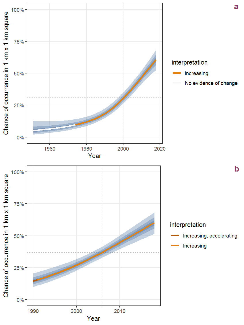
Figure R.76: Effect of year on the probability of Sedum album L. presence in 1 km x 1 km squares where the species has been observed at least once. The fitted line shows the sum of the overall mean (the intercept), a conditional effect of list-length equal to 130 and the year-smoother. The vertical dashed lines indicate the year(s) where the year-smoother is zero. The 95% confidence band is shown in grey (including the variability around the intercept and the smoother). a: 1950 - 2018, b: 1990 - 2018.
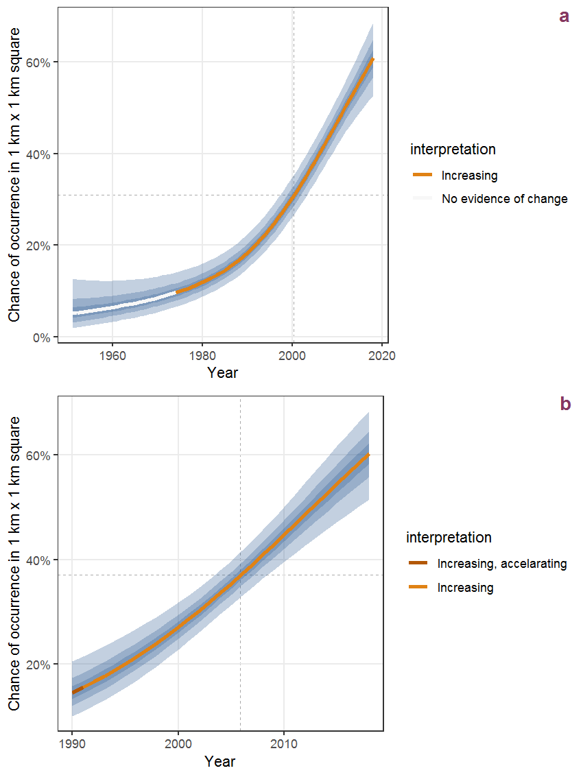
Figure R.77: The same as R.76, but the vertical axis is scaled to the range of the predicted values such that relative changes can be seen more easily. a: 1950 - 2018, b: 1990 - 2018.
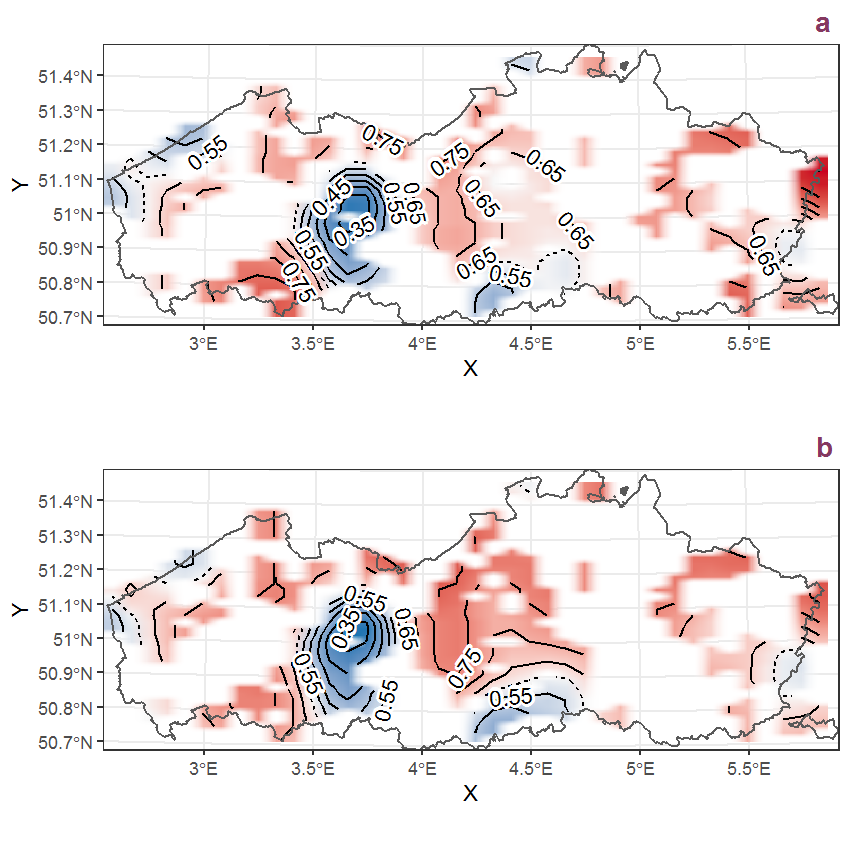
Figure R.78: Visualisation of the spatial smooth effect on the probability of Sedum album L. presence in 1 km x 1 km squares where the species has been observed at least once. The probabilities (values on the contour lines) are conditional on the final year of observation and a list-length equal to 130. The dashed contour line demarcates zones where the species is expected to be more prevalent (red shades) from zones where the species is less prevalent (blue shades). a: 1950 - 2018, b: 1990 - 2018.
R.27 Sedum telephium L.
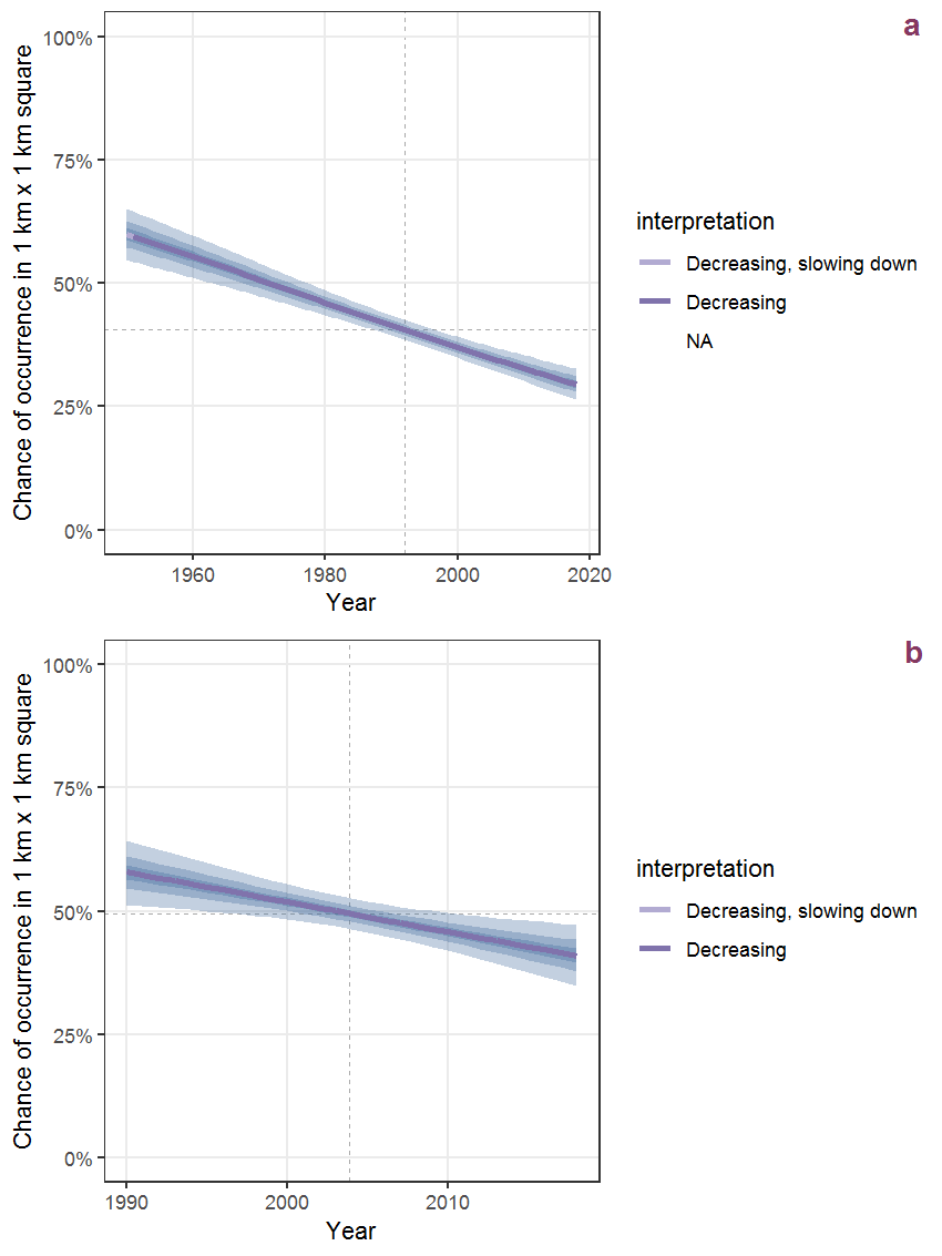
Figure R.79: Effect of year on the probability of Sedum telephium L. presence in 1 km x 1 km squares where the species has been observed at least once. The fitted line shows the sum of the overall mean (the intercept), a conditional effect of list-length equal to 130 and the year-smoother. The vertical dashed lines indicate the year(s) where the year-smoother is zero. The 95% confidence band is shown in grey (including the variability around the intercept and the smoother). a: 1950 - 2018, b: 1990 - 2018.
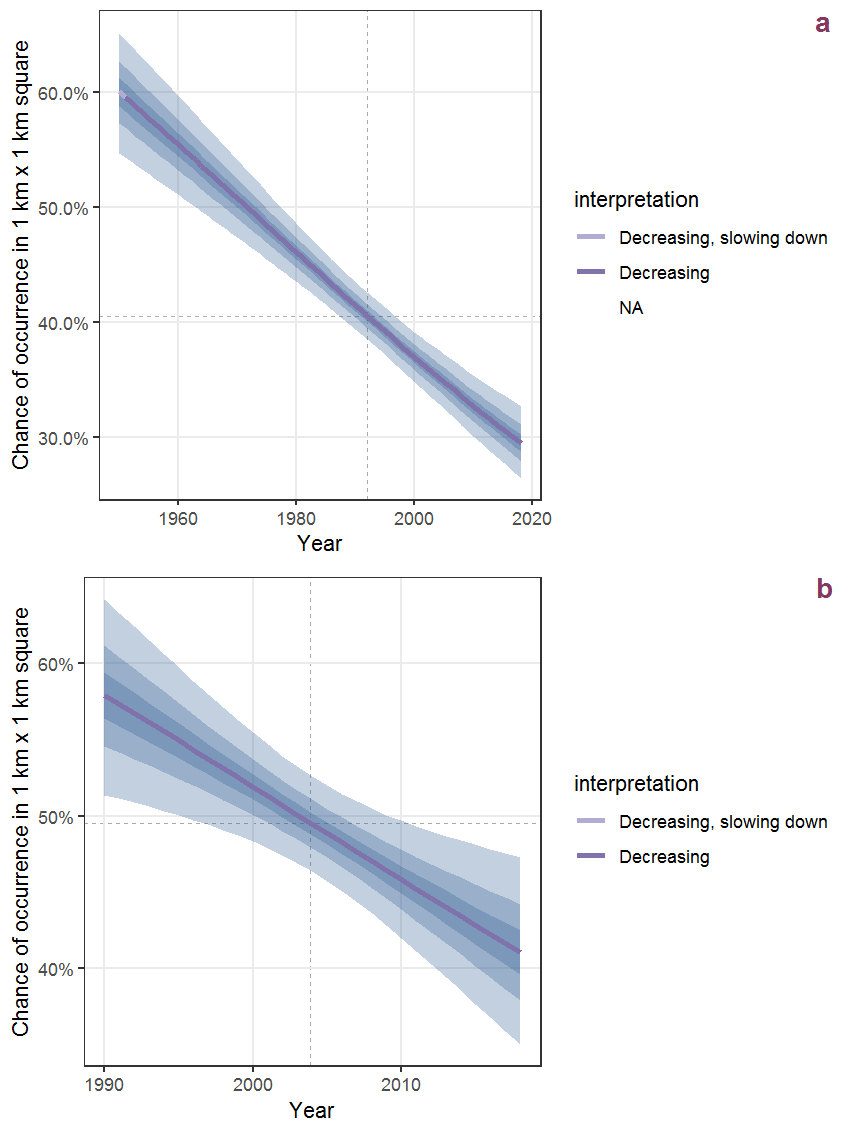
Figure R.80: The same as R.79, but the vertical axis is scaled to the range of the predicted values such that relative changes can be seen more easily. a: 1950 - 2018, b: 1990 - 2018.
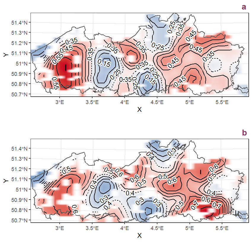
Figure R.81: Visualisation of the spatial smooth effect on the probability of Sedum telephium L. presence in 1 km x 1 km squares where the species has been observed at least once. The probabilities (values on the contour lines) are conditional on the final year of observation and a list-length equal to 130. The dashed contour line demarcates zones where the species is expected to be more prevalent (red shades) from zones where the species is less prevalent (blue shades). a: 1950 - 2018, b: 1990 - 2018.
R.28 Senecio erucifolius L.
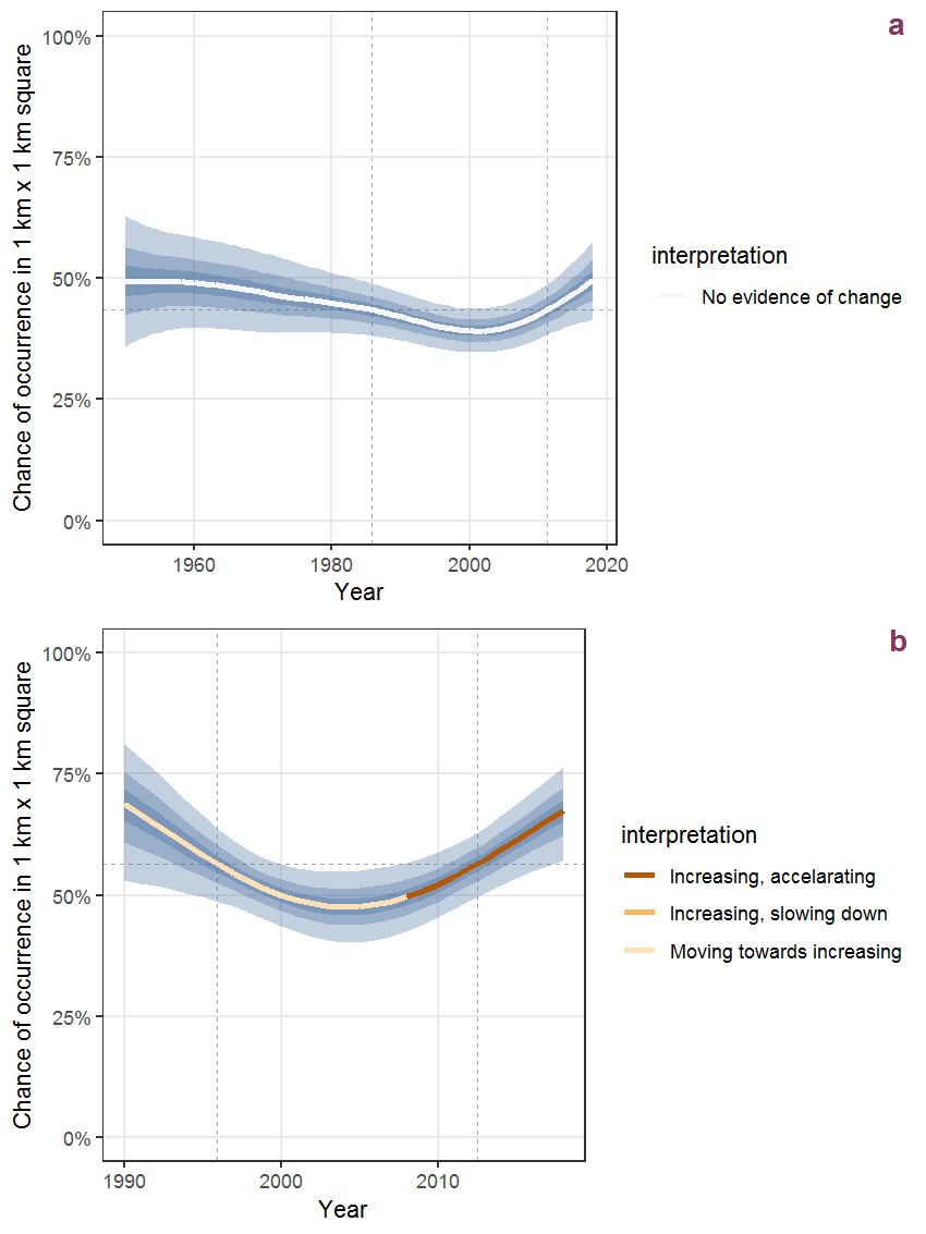
Figure R.82: Effect of year on the probability of Senecio erucifolius L. presence in 1 km x 1 km squares where the species has been observed at least once. The fitted line shows the sum of the overall mean (the intercept), a conditional effect of list-length equal to 130 and the year-smoother. The vertical dashed lines indicate the year(s) where the year-smoother is zero. The 95% confidence band is shown in grey (including the variability around the intercept and the smoother). a: 1950 - 2018, b: 1990 - 2018.
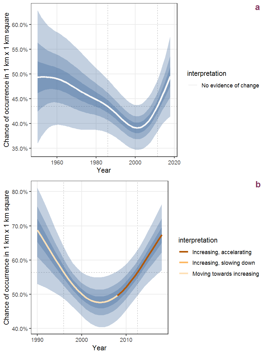
Figure R.83: The same as R.82, but the vertical axis is scaled to the range of the predicted values such that relative changes can be seen more easily. a: 1950 - 2018, b: 1990 - 2018.
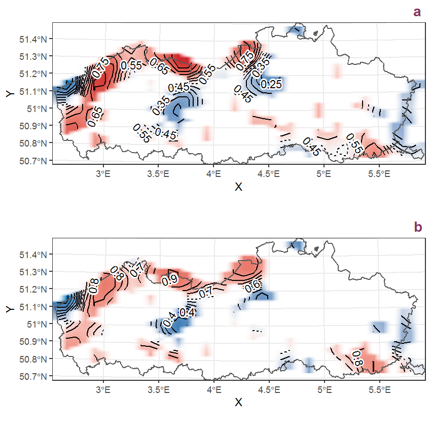
Figure R.84: Visualisation of the spatial smooth effect on the probability of Senecio erucifolius L. presence in 1 km x 1 km squares where the species has been observed at least once. The probabilities (values on the contour lines) are conditional on the final year of observation and a list-length equal to 130. The dashed contour line demarcates zones where the species is expected to be more prevalent (red shades) from zones where the species is less prevalent (blue shades). a: 1950 - 2018, b: 1990 - 2018.
R.29 Senecio inaequidens DC.
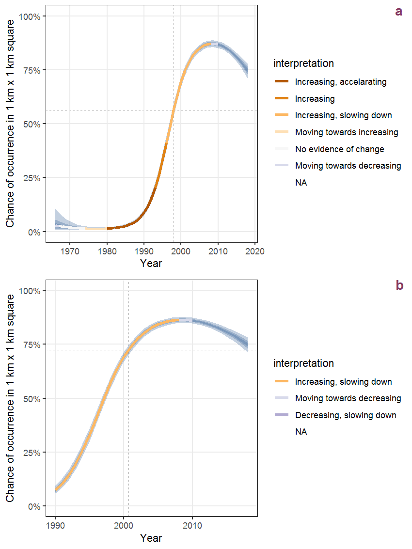
Figure R.85: Effect of year on the probability of Senecio inaequidens DC. presence in 1 km x 1 km squares where the species has been observed at least once. The fitted line shows the sum of the overall mean (the intercept), a conditional effect of list-length equal to 130 and the year-smoother. The vertical dashed lines indicate the year(s) where the year-smoother is zero. The 95% confidence band is shown in grey (including the variability around the intercept and the smoother). a: 1950 - 2018, b: 1990 - 2018.
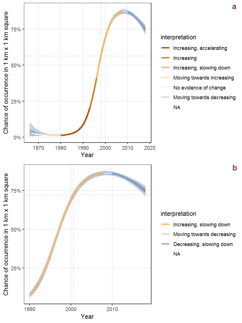
Figure R.86: The same as R.85, but the vertical axis is scaled to the range of the predicted values such that relative changes can be seen more easily. a: 1950 - 2018, b: 1990 - 2018.
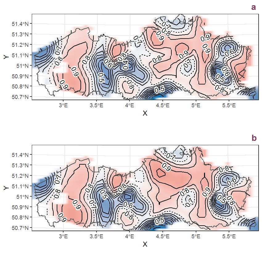
Figure R.87: Visualisation of the spatial smooth effect on the probability of Senecio inaequidens DC. presence in 1 km x 1 km squares where the species has been observed at least once. The probabilities (values on the contour lines) are conditional on the final year of observation and a list-length equal to 130. The dashed contour line demarcates zones where the species is expected to be more prevalent (red shades) from zones where the species is less prevalent (blue shades). a: 1950 - 2018, b: 1990 - 2018.
R.30 Senecio jacobaea L.
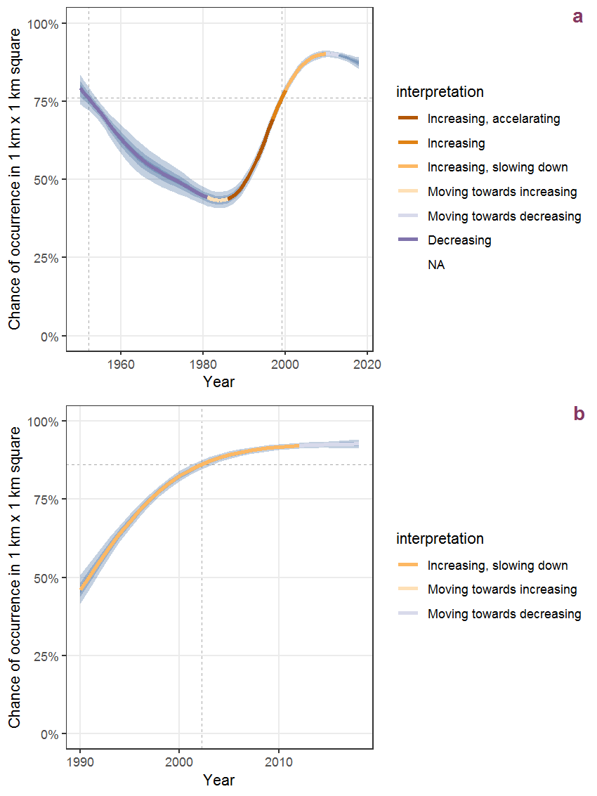
Figure R.88: Effect of year on the probability of Senecio jacobaea L. presence in 1 km x 1 km squares where the species has been observed at least once. The fitted line shows the sum of the overall mean (the intercept), a conditional effect of list-length equal to 130 and the year-smoother. The vertical dashed lines indicate the year(s) where the year-smoother is zero. The 95% confidence band is shown in grey (including the variability around the intercept and the smoother). a: 1950 - 2018, b: 1990 - 2018.
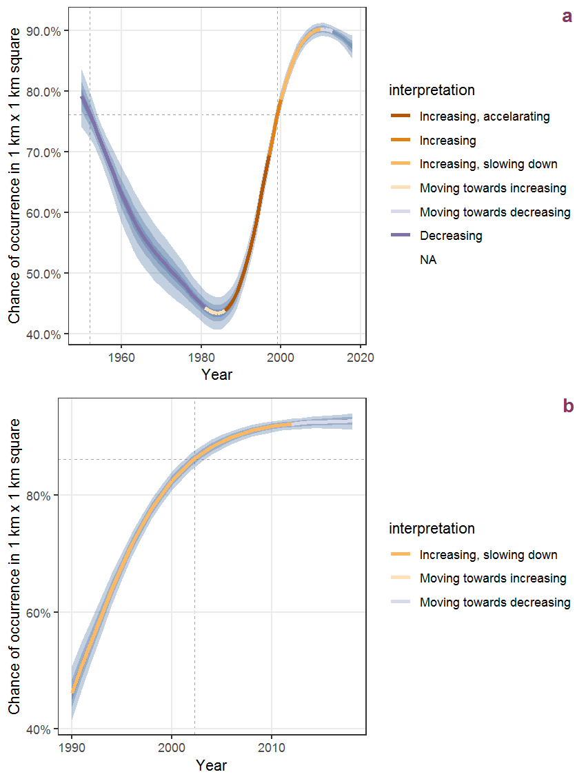
Figure R.89: The same as R.88, but the vertical axis is scaled to the range of the predicted values such that relative changes can be seen more easily. a: 1950 - 2018, b: 1990 - 2018.
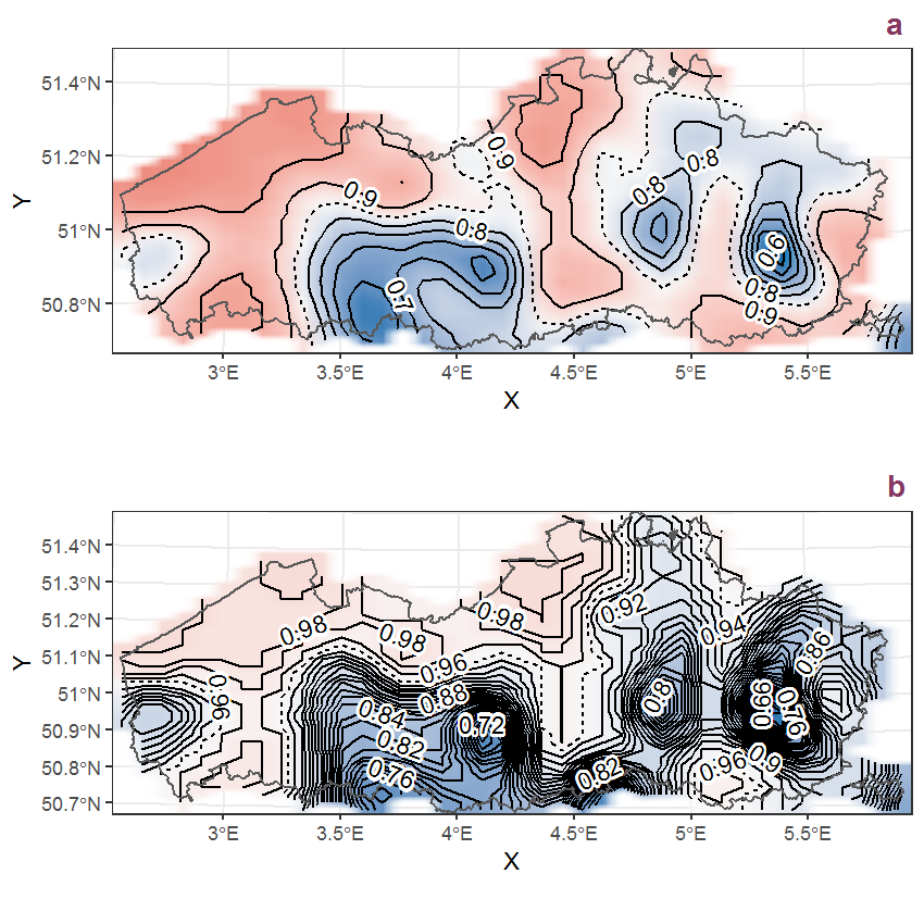
Figure R.90: Visualisation of the spatial smooth effect on the probability of Senecio jacobaea L. presence in 1 km x 1 km squares where the species has been observed at least once. The probabilities (values on the contour lines) are conditional on the final year of observation and a list-length equal to 130. The dashed contour line demarcates zones where the species is expected to be more prevalent (red shades) from zones where the species is less prevalent (blue shades). a: 1950 - 2018, b: 1990 - 2018.
R.31 Senecio ovatus (P. Gaertn., B. Mey. et Scherb.) Willd.
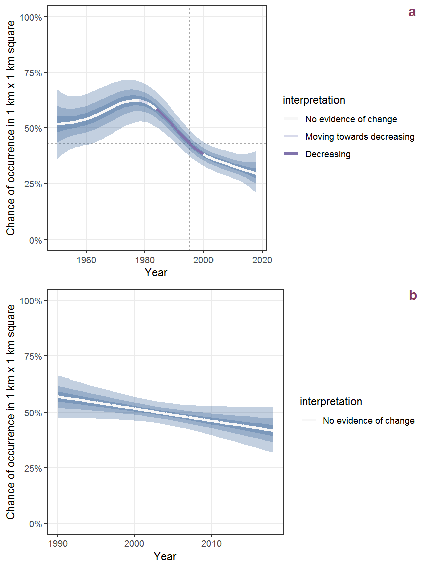
Figure R.91: Effect of year on the probability of Senecio ovatus (P. Gaertn., B. Mey. et Scherb.) Willd. presence in 1 km x 1 km squares where the species has been observed at least once. The fitted line shows the sum of the overall mean (the intercept), a conditional effect of list-length equal to 130 and the year-smoother. The vertical dashed lines indicate the year(s) where the year-smoother is zero. The 95% confidence band is shown in grey (including the variability around the intercept and the smoother). a: 1950 - 2018, b: 1990 - 2018.
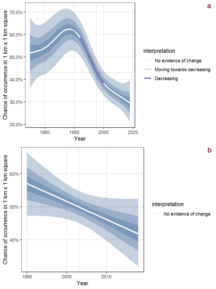
Figure R.92: The same as R.91, but the vertical axis is scaled to the range of the predicted values such that relative changes can be seen more easily. a: 1950 - 2018, b: 1990 - 2018.
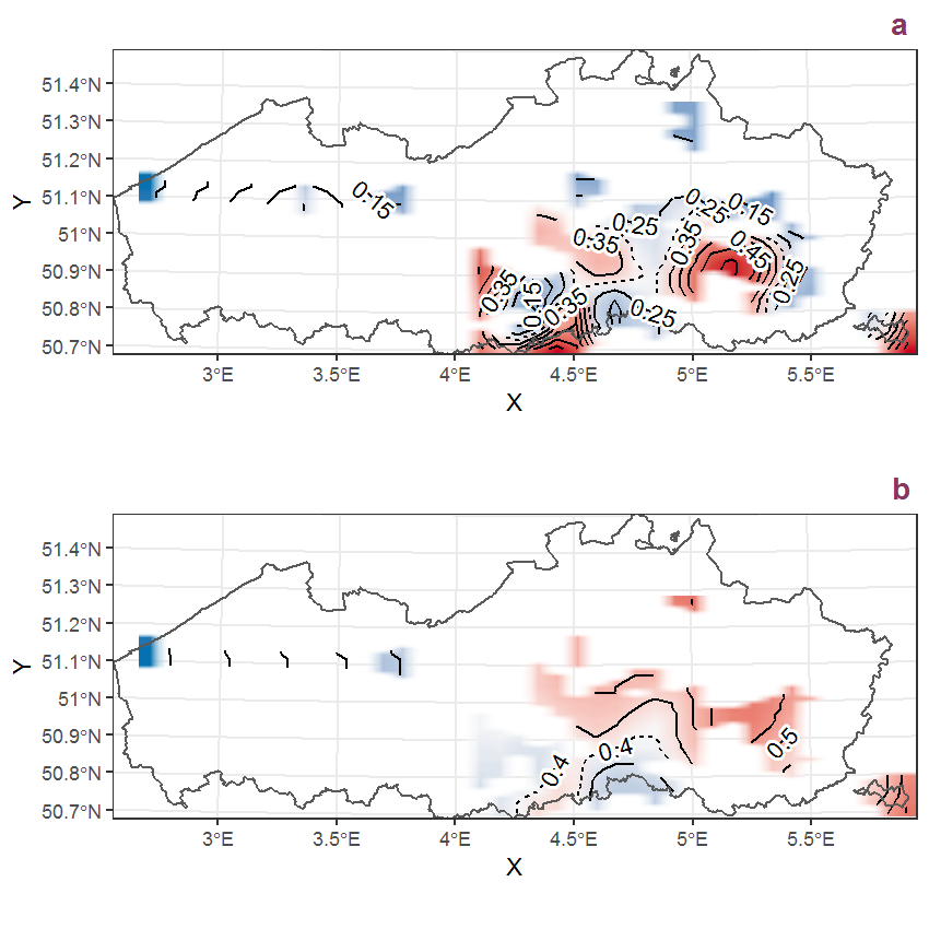
Figure R.93: Visualisation of the spatial smooth effect on the probability of Senecio ovatus (P. Gaertn., B. Mey. et Scherb.) Willd. presence in 1 km x 1 km squares where the species has been observed at least once. The probabilities (values on the contour lines) are conditional on the final year of observation and a list-length equal to 130. The dashed contour line demarcates zones where the species is expected to be more prevalent (red shades) from zones where the species is less prevalent (blue shades). a: 1950 - 2018, b: 1990 - 2018.
R.32 Senecio sylvaticus L.
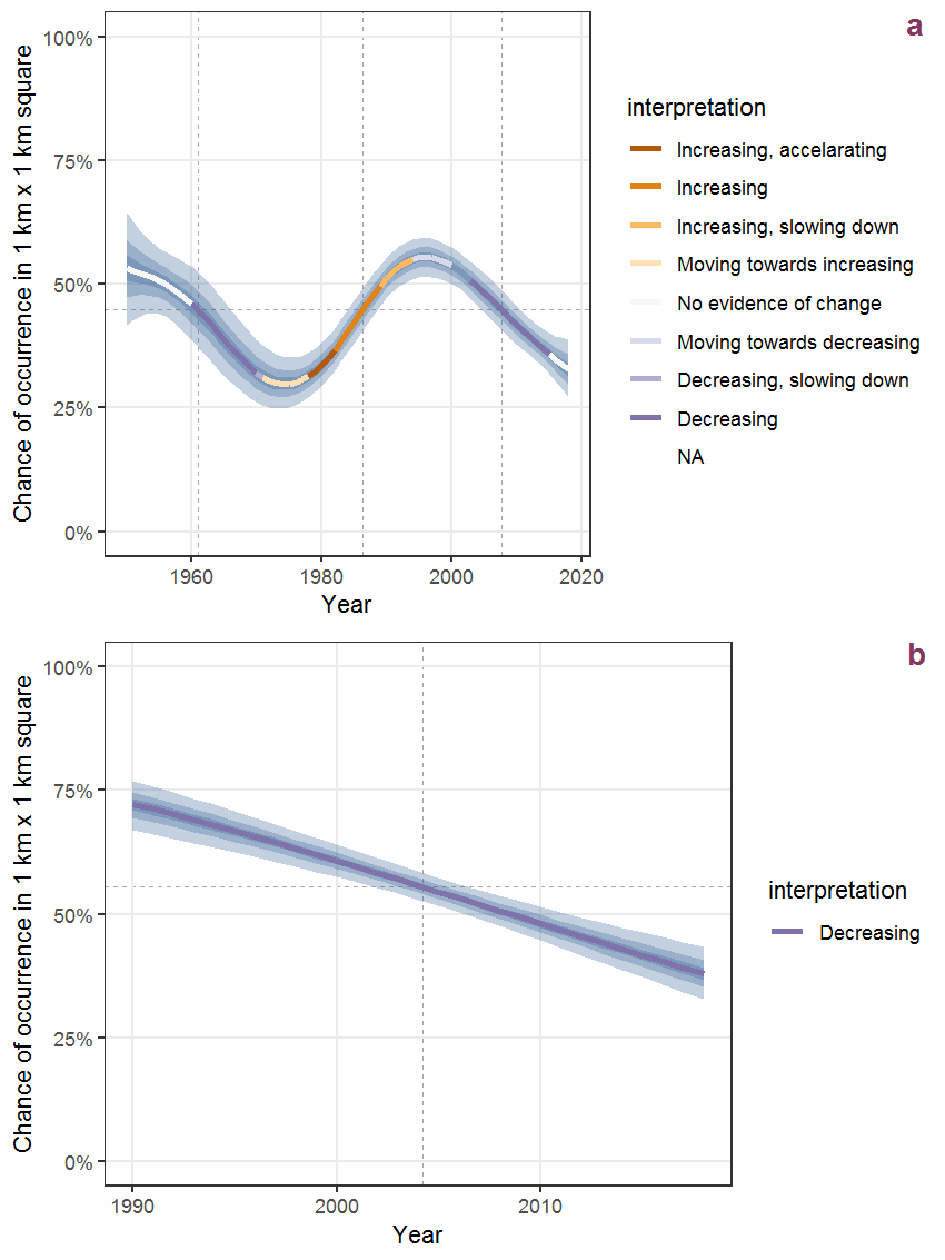
Figure R.94: Effect of year on the probability of Senecio sylvaticus L. presence in 1 km x 1 km squares where the species has been observed at least once. The fitted line shows the sum of the overall mean (the intercept), a conditional effect of list-length equal to 130 and the year-smoother. The vertical dashed lines indicate the year(s) where the year-smoother is zero. The 95% confidence band is shown in grey (including the variability around the intercept and the smoother). a: 1950 - 2018, b: 1990 - 2018.
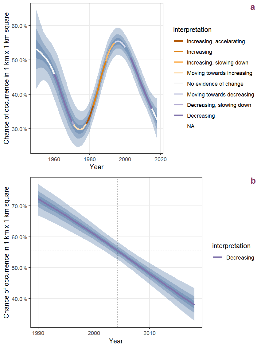
Figure R.95: The same as R.94, but the vertical axis is scaled to the range of the predicted values such that relative changes can be seen more easily. a: 1950 - 2018, b: 1990 - 2018.
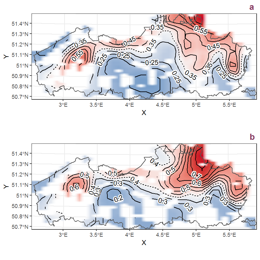
Figure R.96: Visualisation of the spatial smooth effect on the probability of Senecio sylvaticus L. presence in 1 km x 1 km squares where the species has been observed at least once. The probabilities (values on the contour lines) are conditional on the final year of observation and a list-length equal to 130. The dashed contour line demarcates zones where the species is expected to be more prevalent (red shades) from zones where the species is less prevalent (blue shades). a: 1950 - 2018, b: 1990 - 2018.