Getting started
Interactive usage
Niche Vlaanderen can be used interactively in Python. For interactive use, we recommend using the Jupyter notebook. This allows one to save documentation, code and results in the same file.
This file itself is a notebook, and if you want to reproduce our result this is possible:
Download the niche sourcecode (use the zip file).
Extract the file and navigate to the
docsfolder from the anaconda prompt. Make sure you also extract the testcases directory, as this contains the data we will be using.Activate the niche environment:
conda activate niche(not necessary if you used the alternative install).Run Jupyter notebook:
jupyter notebook. This should open a web page (similar or equal to http://localhost:8888 ) - check your anaconda prompt for a link if this is not the case.Navigate your web browser to the
getting_started.ipynbfile (in the Files tab, which should be opened by default).Any cell with code can be run by by pressing Ctrl+Enter. If you are unfamiliar with notebooks, you can take some time familiarizing yourself by taking the User interface tour from the
Helpmenu.
Steps to create a Niche model
To calculate a Niche model one has to take the following steps:
Initialize the model (create a
Nicheobject)Add the different input grids (or constant values) to the model (
set_inputmethod)Run the model (
runmethod)Optionally inspect the results using
plot()andtable.Save the results (
writemethod).
These steps are mirrored in the design of the Niche class which is given below.
Optionally the user can also create difference maps showing how much MHW/MLW has to change to allow a certain vegetation type. This is done using the deviation parameter of the run method.
[1]:
from pathlib import Path
Creating a simple NICHE model
For our first example, we will be creating a simple model, using only MHW, MLW and soil for the predictions.
The first step is importing the niche_vlaanderen module. For convenience, we will be importing as nv.
[2]:
import niche_vlaanderen as nv
Creating a niche object
Next we create a Niche object. This object will hold all the data and results for an analysis.
[3]:
simple = nv.Niche()
Adding input files
After initialization, we can add input layers to this object, using the set_input method.
[4]:
simple.set_input("mhw", "../testcase/zwarte_beek/input/mhw.asc")
simple.set_input("mlw", "../testcase/zwarte_beek/input/mlw.asc")
simple.set_input("soil_code", "../testcase/zwarte_beek/input/soil_code.asc")
Running the model
These three input files are the only required for running a simple NICHE model. This means we can already run our model.
[5]:
simple.run(full_model=False)
Inspecting the model
After a model is run, we can inspect the results using the table method. Note that the values are given in ha. In the example below we also use the head function to show only the first five rows.
[6]:
simple.table.head()
[6]:
| vegetation | presence | area_ha | |
|---|---|---|---|
| 0 | 1 | no data | 15.16 |
| 1 | 1 | not present | 14.44 |
| 2 | 1 | present | 9.88 |
| 3 | 2 | no data | 15.16 |
| 4 | 2 | present | 12.80 |
The returned object is a Pandas dataframe which makes it easy to manipulate (for example calculating a crosstabulation, filtering, …) or save it to a file. Below we present two examples which can be useful when working with these data. The first is saving the data to a csv file.
[7]:
simple.table.to_csv("demo.csv")
By using the pandas pivot_table method, we can create a summarized table. Note that only the first 5 rows are shown because we use the head function
[8]:
result = simple.table.pivot_table(index="vegetation",
                            values="area_ha",
                            columns="presence",
                            fill_value=0).head()

result
[8]:
| presence | no data | not present | present |
|---|---|---|---|
| vegetation | |||
| 1 | 15.16 | 14.44 | 9.88 |
| 2 | 15.16 | 11.52 | 12.80 |
| 3 | 15.16 | 5.88 | 18.44 |
| 4 | 15.16 | 21.16 | 3.16 |
| 5 | 15.16 | 24.32 | 0.00 |
It is also possible to show actual grids using the plot method.
[9]:
%matplotlib inline
import matplotlib.pyplot as plt

ax = simple.plot(11)
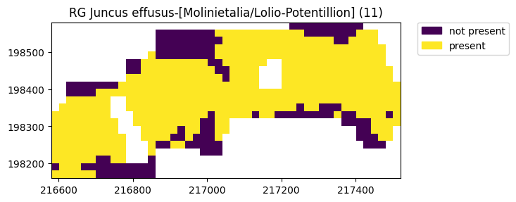
It is possible to give your model a name - this will be shown when plotting and will be used when writing the files.
[10]:
simple.name="scen_1"
ax = simple.plot(11)

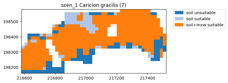
Rather than showing just the presence, a detailed plot will also show why certain parts are not present
[11]:
ax = simple.plot_detail(7)
Saving the model
The model results can be saved to disk using the write function. As an argument, this takes the directory to which you want to save, _output_scen1 in our example. When saving a model, the log file, containing the model configuration, a summary table and all 28 vegetation grids will be saved. Note we specify the overwrite_files option so subsequent calls of the example will not raise an error
[12]:
simple.write("_output_scen1", overwrite_files=True)
Below you can see the list of files that is generated by this operation: There are the 28 vegetation grids (*.tif files), the summary table (summary.csv) and a logfile (log.txt). All files are prepended with the model name we set earlier.
[13]:
import os
sorted(os.listdir("_output_scen1"))
[13]:
['scen_1_V01.tif',
 'scen_1_V02.tif',
 'scen_1_V03.tif',
 'scen_1_V04.tif',
 'scen_1_V05.tif',
 'scen_1_V06.tif',
 'scen_1_V07.tif',
 'scen_1_V08.tif',
 'scen_1_V09.tif',
 'scen_1_V10.tif',
 'scen_1_V11.tif',
 'scen_1_V12.tif',
 'scen_1_V13.tif',
 'scen_1_V14.tif',
 'scen_1_V15.tif',
 'scen_1_V16.tif',
 'scen_1_V17.tif',
 'scen_1_V18.tif',
 'scen_1_V19.tif',
 'scen_1_V20.tif',
 'scen_1_V21.tif',
 'scen_1_V22.tif',
 'scen_1_V23.tif',
 'scen_1_V24.tif',
 'scen_1_V25.tif',
 'scen_1_V26.tif',
 'scen_1_V27.tif',
 'scen_1_V28.tif',
 'scen_1_log.txt',
 'scen_1_summary.csv']
Showing the model configuration
While using niche, it is always possible to view the configuration by typing the object name.
[14]:
simple
[14]:
# Niche Vlaanderen version: 2.0
# Using latest niche_vlaanderen  2.0
# Reference values:
#     version: 12C
#     source: 10.5281/zenodo.10521548
#     original file: NICHE_FL_referencegroundwaterlevels_v12C.csv
# Run at: 2024-10-31 09:55:52.017933

package_versions:
  pandas: 2.2.2
  numpy: 1.26.4
  rasterio: 1.3.10
  gdal: 3.8.4
  python: '3.11.0 | packaged by conda-forge | (main, Jan 14 2023, 12:27:40) [GCC 11.3.0]'

model_options:
  deviation: false
  full_model: false
  name: scen_1
  output_dir: _output_scen1
  strict_checks: true

model_properties:
  model_extent: ((216580.0, 198580.0), (217520.0, 198160.0))

input_layers:
  mhw: ../testcase/zwarte_beek/input/mhw.asc
  mlw: ../testcase/zwarte_beek/input/mlw.asc
  soil_code: ../testcase/zwarte_beek/input/soil_code.asc
  # Model run completed
files_written:
  1: _output_scen1/scen_1_V01.tif
  2: _output_scen1/scen_1_V02.tif
  3: _output_scen1/scen_1_V03.tif
  4: _output_scen1/scen_1_V04.tif
  5: _output_scen1/scen_1_V05.tif
  6: _output_scen1/scen_1_V06.tif
  7: _output_scen1/scen_1_V07.tif
  8: _output_scen1/scen_1_V08.tif
  9: _output_scen1/scen_1_V09.tif
  10: _output_scen1/scen_1_V10.tif
  11: _output_scen1/scen_1_V11.tif
  12: _output_scen1/scen_1_V12.tif
  13: _output_scen1/scen_1_V13.tif
  14: _output_scen1/scen_1_V14.tif
  15: _output_scen1/scen_1_V15.tif
  16: _output_scen1/scen_1_V16.tif
  17: _output_scen1/scen_1_V17.tif
  18: _output_scen1/scen_1_V18.tif
  19: _output_scen1/scen_1_V19.tif
  20: _output_scen1/scen_1_V20.tif
  21: _output_scen1/scen_1_V21.tif
  22: _output_scen1/scen_1_V22.tif
  23: _output_scen1/scen_1_V23.tif
  24: _output_scen1/scen_1_V24.tif
  25: _output_scen1/scen_1_V25.tif
  26: _output_scen1/scen_1_V26.tif
  27: _output_scen1/scen_1_V27.tif
  28: _output_scen1/scen_1_V28.tif
Note that this overview contains the same information as the logfile which we wrote before. Later on, we will show that this can be used as input when running Niche with a configuration file (either from within Python or from the command line).
Running a full Niche model
A full Niche model requires more inputs that only mhw, mlw and soil_code. The full list can be found in the documentation. When trying to run a model without sufficient inputs, a warning will be generated.
If we add all the required values, we can run the full model. Note that it is possible to set a constant value instead of a complete grid
[15]:
full = nv.Niche()
input_folder = Path("../testcase/zwarte_beek/input/")
full.set_input("mhw", input_folder / "mhw.asc")
full.set_input("mlw", input_folder / "mlw.asc")
full.set_input("soil_code", input_folder / "soil_code.asc")
full.set_input("nitrogen_animal", 0)
full.set_input("inundation_acidity", input_folder / "inundation.asc")
full.set_input("inundation_nutrient", input_folder / "inundation.asc")
full.set_input("nitrogen_fertilizer",0)
full.set_input("minerality", input_folder / "minerality.asc")
full.set_input("management", input_folder / "management.asc")
full.set_input("nitrogen_atmospheric", 0)
full.set_input("msw", input_folder / "msw.asc")
full.set_input("rainwater", 0)
full.set_input("seepage", input_folder / "seepage.asc")
full.run()
We can look at the full model using the same table and plot functions as we used for the simple model.
[16]:
full.table.head()
[16]:
| vegetation | presence | area_ha | |
|---|---|---|---|
| 0 | 1 | not present | 15.44 |
| 1 | 1 | no data | 15.16 |
| 2 | 1 | present | 8.88 |
| 3 | 2 | not present | 21.52 |
| 4 | 2 | no data | 15.16 |
Comparing to the simple model, one can observe that the area where a vegetation type can be present is always smaller than in the simple model.
[17]:
simple.table.head()
[17]:
| vegetation | presence | area_ha | |
|---|---|---|---|
| 0 | 1 | no data | 15.16 |
| 1 | 1 | not present | 14.44 |
| 2 | 1 | present | 9.88 |
| 3 | 2 | no data | 15.16 |
| 4 | 2 | present | 12.80 |
In the next tutorial, we will focus on more advanced methods for using the package, starting with the comparison of these two models.