Advanced usage

Using config files

Instead of specifying all inputs using set_input, it is possible to use a config file. A config file can be loaded using read_config_file or it can be read and executed immediately by using run_config_file.

The syntax of the config file is explained more in detail in Niche Configuration file, but is already introduced here because it will be used in the next examples.

If you want to recreate the examples below, the config files can be found under the docs folder, so if you extract all the data the you should be able to run the examples from the notebook.

Comparing Niche classes

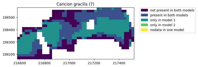
Niche models can be compared using a NicheDelta class. This can be used to compare different scenario’s.

In our example, we will compare the results of the running Niche two times, once using a simple model and once using a full model.

[1]:

import niche_vlaanderen as nv
import matplotlib.pyplot as plt

simple = nv.Niche()
simple.run_config_file("simple.yml")

full = nv.Niche()
full.run_config_file("full.yml")

delta = nv.NicheDelta(simple, full)
ax = delta.plot(7)
plt.show()

It is also possible to show the areas in a dataframe by using the table attribute.

[2]:

delta.table.head()

[2]:

	vegetation	presence	area_ha
0	1	not present in both models	14.44
1	1	present in both models	8.88
2	1	only in model 1	1.00
3	2	not present in both models	11.52
4	2	only in model 1	10.00

Like Niche, NicheDelta also has a write method, which takes a directory as an argument.

[3]:

delta.write("comparison_output", overwrite_files=True)

Creating deviation maps

In many cases, it is not only important to find out which vegetation types are possible given the different input files, but also to find out how much change would be required to mhw or mlw to allow a certain vegetation type.

To create deviation maps, it is necessary to run a model with the deviation option.

[4]:

dev = nv.Niche()
dev.set_input("mhw","../testcase/zwarte_beek/input/mhw.asc")
dev.set_input("mlw","../testcase/zwarte_beek/input/mhw.asc")
dev.set_input("soil_code","../testcase/zwarte_beek/input/soil_code.asc")
dev.run(deviation=True, full_model=False)

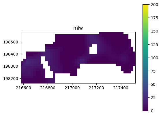
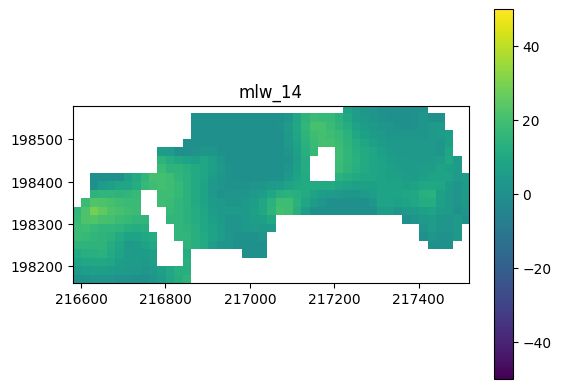
The deviation maps can be plotted by specifying either mhw or mlw with the vegetation type, eg mhw_14 (to show the deviation between mhw and the required mhw for vegetation type 14). Positive values indicate that the actual condition is too dry for the vegetation type. Negative values indicate that the actual condition is too wet for the vegetation type.

[5]:

dev.plot("mlw")
dev.plot("mlw_14")

plt.show()

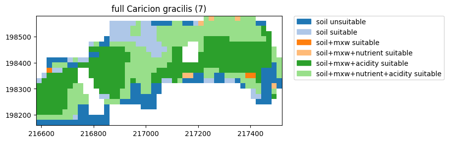
Create detailed absence/presence plots

Rather than just showing if a certain vegetation type is present or not present, it is possible to show a more detailed analysis on the reason a vegetation type is present or not present. This follows the steps of the niche analysis: ie if soil type is possible, mxw checks are done and finally other input grids are matched.

[6]:

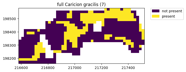
ax = full.plot(7)
ax = full.plot_detail(7)

This detailed version of the map can be exported with:

[7]:

full.write("output", detailed_files=True)

Creating statistics per shape object

Niche also contains a helper function that allows one to calculate the possible vegetation by using a vector dataset, such as a .geojson or .shp file.

The vegetation is returned as a pandas dataframe, where shapes are identified by their id and the area not covered by a shape gets shape_id -1.

[8]:

df = full.zonal_stats("../testcase/zwarte_beek/input/study_area_l72.geojson")
df

100%|██████████████████████████████████████████████████████████████████████████████████████████████████████| 28/28 [00:00<00:00, 160.68it/s]

[8]:

	vegetation	shape_id	presence	area_ha
0	1	0	not present	15.44
1	1	0	present	8.88
2	1	0	no data	0.00
3	2	0	not present	21.52
4	2	0	present	2.80
...	...	...	...	...
79	15	-1	present	0.00
80	16	-1	present	0.00
81	20	-1	present	0.00
82	21	-1	present	0.00
83	28	-1	present	0.00

168 rows × 4 columns

Using abiotic grids

In certain cases the intermediary grids of Acidity or NutrientLevel need changes, to compensate for specific circumstances.

In that case it is possible to run a Niche model and make some adjustments to the grid and then using an abiotic grid as an input.

[9]:

import niche_vlaanderen as nv
import matplotlib.pyplot as plt

full = nv.Niche()
full.run_config_file("full.yml")
full.write("output_abiotic", overwrite_files=True)

Now it is possible to adapt the acidity and nutrient_level grids outside niche. For this demo, we will use some Python magic to make all nutrient levels one level lower. Note that there is no need to do this in Python, any other tool could be used as well. So if you don’t understand this code - don’t panic (and ignore the warning)!

[10]:

import rasterio
with rasterio.open("output_abiotic/full_nutrient_level.tif") as src:
    nutrient_level = src.read(1)
    profile = src.profile
    nodata = src.nodatavals[0]

nutrient_level[nutrient_level != nodata] = nutrient_level[nutrient_level != nodata] -1

# we can not have nutrient level 0, so we set all places where this occurs to 1
nutrient_level[nutrient_level ==0 ] = 1

with rasterio.open("output_abiotic/adjusted_nutrient.tif", 'w', **profile) as dst:
    dst.write(nutrient_level, 1)

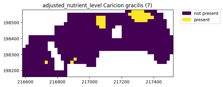
Next we will create a new niche model using the same options as our previous full models, but we will add the previously calculated nutrient level as input: in this case, this nutrient level grid will be used (and not calculated from the other grids). Note that we use the read_config_file method (and not run_config_file) because we still want to edit the configuration before running.

[11]:

adjusted = nv.Niche()
# set the input layers as usual:
adjusted.read_config_file("full.yml")
# now select a custom layer for the nutrient level:
adjusted.set_input("nutrient_level", "output_abiotic/adjusted_nutrient.tif")
# since we do not define a custom acidity layer to use, acidity will be calculated as usual
adjusted.name = "adjusted_nutrient_level"
adjusted.run()

adjusted.plot(7)
full.plot(7)
plt.show()

Overwriting standard code tables

One is free to adapt the standard code tables that are used by NICHE. By specifying the paths to the adapted code tables in a NICHE class object, the standard code tables can be overwritten. In this way, standard model functioning can be tweaked. However, it is strongly advised to use ecological data that is reviewed by experts and to have in-depth knowledge of the model functioning.

The possible code tables that can be adapted and set within a NICHE object are:

ct_acidity, ct_soil_mlw_class, ct_soil_codes, lnk_acidity, ct_seepage, ct_vegetation, ct_management, ct_nutrient_level and ct_mineralisation

After adapting the vegetation code table for type 7 (Caricion gracilis) on peaty soil (V) by randomly altering the maximum mhw and mlw to 5 and 4 cm resp. (i.e. below ground, instead of standard values of -28 and -29 cm) and saving the file to ct_vegetation_adj7.csv, the adjusted model can be built and run.

[12]:

adjusted_ct = nv.Niche(ct_vegetation = "ct_vegetation_adj7.csv")
adjusted_ct.read_config_file("full.yml")
adjusted_ct.run()

Example of changed potential area of Caricion gracilis vegetation type because of the changes set in the vegetation code table:

[13]:

adjusted_ct.plot(7)
full.plot(7)
plt.show()

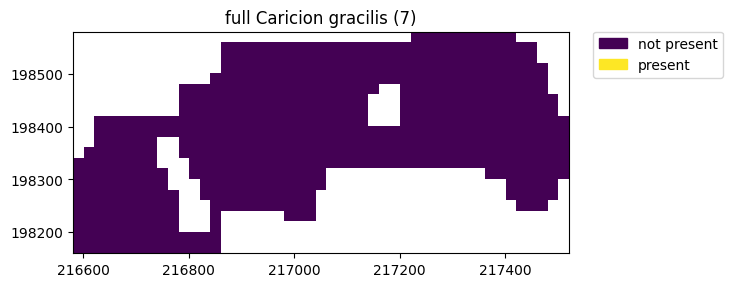
Potential area is shrinking because of the range of grondwater levels that have become more narrow (excluding the wettest places).