Coordinate operations and maps in R
This tutorial shows how to do coordinate transformations and conversions in R. It also demonstrates how spatial data can be mapped with ggplot2 and mapview.
Introduction and setup
This tutorial originated while preparing an R-demonstration during a GIS club at INBO on 16 September 2021. (Further material of the GIS club is available here.)
A straightforward approach for transforming spatial data is available in another tutorial. The current tutorial tackles a few extra aspects.
The tutorial assumes you have some pre-existing knowledge:
- Basic knowledge about coordinate reference systems (CRSs) and geodetic datums; see another tutorial and the references and links therein.
- Knowing how to read geospatial files with
sf. There is another tutorial demonstrating some aspects.
In this tutorial we will apply conversions (without datum shift) and
transformations (with datum shift) to sf and sfc objects. In the
background, these operations use the PROJ library.
Let’s load the needed R packages and prepare a more appropriate theme
for mapping with ggplot2:
library(dplyr)
library(sf)
library(ggplot2)
theme_set(theme_bw())
theme_update(panel.grid = element_line(colour = "grey80"))
library(mapview)
Set up input data if needed:
if (!file.exists(file.path(gisclubdata_path, "gemeenten_belgie.shp"))) {
  googledrive::drive_download(googledrive::as_id("1-epL-fyKB8eS-WwuZhjsl8uyZYplAqFA"),
                              file.path(tempdir(), "data_gisclub.zip"))
  unzip(file.path(tempdir(), "data_gisclub.zip"),
        exdir = tempdir())
  list.files(file.path(tempdir(), "data_gisclub"), full.names = TRUE) %>%
    file.copy(gisclubdata_path, recursive = TRUE)
}
The code assumes that you have a gisclubdata_path object defined
(directory path as a string).
Joining and mapping polygon layers
For a given municipalities and watercourses dataset, we would like
to append the municipality name to the watercourses by making a spatial
join.
Reading data and trying to join
Let’s read the data file of Belgian municipalities:
path_municipalities <- file.path(gisclubdata_path, "gemeenten_belgie.shp")
municipalities <- read_sf(path_municipalities)
It looks like this:
municipalities
Simple feature collection with 581 features and 3 fields
Geometry type: MULTIPOLYGON
Dimension:     XYZ
Bounding box:  xmin: 2.541331 ymin: 49.49695 xmax: 6.408098 ymax: 51.50511
z_range:       zmin: 0 zmax: 0
Geodetic CRS:  WGS 84
# A tibble: 581 × 4
   T_MUN_NL        Shape_Leng Shape_Area                                geometry
   <chr>                <dbl>      <dbl>                      <MULTIPOLYGON [°]>
 1 ’s Gravenbrakel      0.759    0.0108  Z (((4.095037 50.66599 0, 4.095101 50.…
 2 Aalst                0.676    0.0101  Z (((4.054666 50.99444 0, 4.054666 50.…
 3 Aalter               0.735    0.0154  Z (((3.41099 51.15987 0, 3.41275 51.15…
 4 Aarlen               0.951    0.0148  Z (((5.860749 49.72667 0, 5.860889 49.…
 5 Aarschot             0.640    0.00807 Z (((4.927684 51.03717 0, 4.92797 51.0…
 6 Aartselaar           0.265    0.00141 Z (((4.401293 51.14814 0, 4.400461 51.…
 7 Aat                  0.977    0.0163  Z (((3.756864 50.69743 0, 3.757621 50.…
 8 Affligem             0.261    0.00229 Z (((4.114181 50.92559 0, 4.115272 50.…
 9 Aiseau-Presles       0.393    0.00284 Z (((4.584122 50.43827 0, 4.584458 50.…
10 Alken                0.336    0.00361 Z (((5.275147 50.9102 0, 5.275645 50.9…
# … with 571 more rows
It appears that the points have three coordinate dimensions (XYZ).
However the features have only two useful dimensions:
st_dimension(municipalities)
  [1] 2 2 2 2 2 2 2 2 2 2 2 2 2 2 2 2 2 2 2 2 2 2 2 2 2 2 2 2 2 2 2 2 2 2 2 2 2
 [38] 2 2 2 2 2 2 2 2 2 2 2 2 2 2 2 2 2 2 2 2 2 2 2 2 2 2 2 2 2 2 2 2 2 2 2 2 2
 [75] 2 2 2 2 2 2 2 2 2 2 2 2 2 2 2 2 2 2 2 2 2 2 2 2 2 2 2 2 2 2 2 2 2 2 2 2 2
[112] 2 2 2 2 2 2 2 2 2 2 2 2 2 2 2 2 2 2 2 2 2 2 2 2 2 2 2 2 2 2 2 2 2 2 2 2 2
[149] 2 2 2 2 2 2 2 2 2 2 2 2 2 2 2 2 2 2 2 2 2 2 2 2 2 2 2 2 2 2 2 2 2 2 2 2 2
[186] 2 2 2 2 2 2 2 2 2 2 2 2 2 2 2 2 2 2 2 2 2 2 2 2 2 2 2 2 2 2 2 2 2 2 2 2 2
[223] 2 2 2 2 2 2 2 2 2 2 2 2 2 2 2 2 2 2 2 2 2 2 2 2 2 2 2 2 2 2 2 2 2 2 2 2 2
[260] 2 2 2 2 2 2 2 2 2 2 2 2 2 2 2 2 2 2 2 2 2 2 2 2 2 2 2 2 2 2 2 2 2 2 2 2 2
[297] 2 2 2 2 2 2 2 2 2 2 2 2 2 2 2 2 2 2 2 2 2 2 2 2 2 2 2 2 2 2 2 2 2 2 2 2 2
[334] 2 2 2 2 2 2 2 2 2 2 2 2 2 2 2 2 2 2 2 2 2 2 2 2 2 2 2 2 2 2 2 2 2 2 2 2 2
[371] 2 2 2 2 2 2 2 2 2 2 2 2 2 2 2 2 2 2 2 2 2 2 2 2 2 2 2 2 2 2 2 2 2 2 2 2 2
[408] 2 2 2 2 2 2 2 2 2 2 2 2 2 2 2 2 2 2 2 2 2 2 2 2 2 2 2 2 2 2 2 2 2 2 2 2 2
[445] 2 2 2 2 2 2 2 2 2 2 2 2 2 2 2 2 2 2 2 2 2 2 2 2 2 2 2 2 2 2 2 2 2 2 2 2 2
[482] 2 2 2 2 2 2 2 2 2 2 2 2 2 2 2 2 2 2 2 2 2 2 2 2 2 2 2 2 2 2 2 2 2 2 2 2 2
[519] 2 2 2 2 2 2 2 2 2 2 2 2 2 2 2 2 2 2 2 2 2 2 2 2 2 2 2 2 2 2 2 2 2 2 2 2 2
[556] 2 2 2 2 2 2 2 2 2 2 2 2 2 2 2 2 2 2 2 2 2 2 2 2 2 2
Some tools – e.g. spherical geoprocessing – expect XY data. So we will
drop the Z dimension with st_zm(). Meanwhile we select the only
necessary attribute and rename it, using select().
municipalities <-
  municipalities %>%
  select(municipality = T_MUN_NL) %>%
  st_zm()
We perform similar operations on the watercourses dataset. Here, data
are already defined as two dimensions.
path_watercourses <- file.path(gisclubdata_path, "watergangen_antw.shp")
watercourses <- read_sf(path_watercourses)
watercourses
Simple feature collection with 7258 features and 14 fields
Geometry type: POLYGON
Dimension:     XY
Bounding box:  xmin: 138050.5 ymin: 201644.5 xmax: 162761.3 ymax: 230509
CRS:           NA
# A tibble: 7,258 × 15
     OIDN   UIDN VERSIE BEGINDATUM VERSDATUM   VHAG NAAM       OPNDATUM   BGNINV
    <dbl>  <dbl>  <int> <date>     <date>     <dbl> <chr>      <date>      <int>
 1 205462 492073      3 2017-07-05 2021-05-06  3320 nvt        2017-06-20     13
 2 179828 488809      2 2015-01-20 2021-05-06    -9 nvt        2014-12-02      4
 3 223031 499842      2 2018-03-28 2021-05-06 54710 Kallebeek… 2018-02-27      4
 4 267383 462960      2 2020-02-22 2021-05-06    -9 nvt        2020-01-08      4
 5  72361 481073      3 2010-11-08 2021-05-06 65101 nvt        2020-06-22      6
 6 223073 499879      3 2018-03-28 2021-05-06    -9 nvt        2018-02-27     13
 7  72079 480970      3 2010-11-08 2021-05-06 53460 nvt        2016-06-20      3
 8 145811 567202      3 2012-11-20 2021-07-07    -8 ng         2012-10-19     11
 9 205453 492064      3 2017-07-05 2021-05-06    -9 nvt        2017-06-20     10
10 269842 463401      2 2020-04-22 2021-05-06    -9 nvt        2020-04-03      4
# … with 7,248 more rows, and 6 more variables: LBLBGNINV <chr>, LENGTE <dbl>,
#   OPPERVL <dbl>, Shape_Leng <dbl>, Shape_Area <dbl>, geometry <POLYGON>
Note that not all columns are printed. Let’s preview all columns with
glimpse():
glimpse(watercourses)
Rows: 7,258
Columns: 15
$ OIDN       <dbl> 205462, 179828, 223031, 267383, 72361, 223073, 72079, 14581…
$ UIDN       <dbl> 492073, 488809, 499842, 462960, 481073, 499879, 480970, 567…
$ VERSIE     <int> 3, 2, 2, 2, 3, 3, 3, 3, 3, 2, 1, 2, 2, 1, 2, 1, 2, 3, 2, 3,…
$ BEGINDATUM <date> 2017-07-05, 2015-01-20, 2018-03-28, 2020-02-22, 2010-11-08…
$ VERSDATUM  <date> 2021-05-06, 2021-05-06, 2021-05-06, 2021-05-06, 2021-05-06…
$ VHAG       <dbl> 3320, -9, 54710, -9, 65101, -9, 53460, -8, -9, -9, -9, -9, …
$ NAAM       <chr> "nvt", "nvt", "Kallebeekgeul", "nvt", "nvt", "nvt", "nvt", …
$ OPNDATUM   <date> 2017-06-20, 2014-12-02, 2018-02-27, 2020-01-08, 2020-06-22…
$ BGNINV     <int> 13, 4, 4, 4, 6, 13, 3, 11, 10, 4, 1, 4, 4, 1, 4, 4, 1, 13, …
$ LBLBGNINV  <chr> "aanmaak uniek percelenplan\r\n", "bijhouding binnengebiede…
$ LENGTE     <dbl> 570.19, 185.33, 1491.01, 307.60, 286.06, 270.32, 48.11, 17.…
$ OPPERVL    <dbl> 2492.23, 494.77, 9350.36, 978.46, 432.97, 405.56, 118.29, 1…
$ Shape_Leng <dbl> 570.18844, 185.32549, 1491.01243, 307.59691, 286.06075, 270…
$ Shape_Area <dbl> 2492.22527, 494.77446, 9350.36080, 978.46010, 432.97004, 40…
$ geometry   <POLYGON> POLYGON ((141976.5 222453.1..., POLYGON ((142200.6 2050…
We only select some:
watercourses <-
  watercourses %>%
  select(polygon_id = OIDN,
         vhag_code = VHAG,
         watercourse = NAAM)
watercourses
Simple feature collection with 7258 features and 3 fields
Geometry type: POLYGON
Dimension:     XY
Bounding box:  xmin: 138050.5 ymin: 201644.5 xmax: 162761.3 ymax: 230509
CRS:           NA
# A tibble: 7,258 × 4
   polygon_id vhag_code watercourse                                     geometry
        <dbl>     <dbl> <chr>                                          <POLYGON>
 1     205462      3320 nvt           ((141976.5 222453.1, 141973.1 222449.6, 1…
 2     179828        -9 nvt           ((142200.6 205085.9, 142197.3 205085, 142…
 3     223031     54710 Kallebeekgeul ((146874.6 203777.1, 146879.3 203775.9, 1…
 4     267383        -9 nvt           ((148997 209136.1, 148996.7 209136.1, 148…
 5      72361     65101 nvt           ((141780.9 213697.8, 141780.7 213695.3, 1…
 6     223073        -9 nvt           ((144377.8 205161.2, 144408.7 205152.8, 1…
 7      72079     53460 nvt           ((140094.1 210962.7, 140093.8 210962.5, 1…
 8     145811        -8 ng            ((149004.6 209659.9, 149002.5 209666.4, 1…
 9     205453        -9 nvt           ((139682 225241.4, 139697.5 225222, 13971…
10     269842        -9 nvt           ((155762.1 207273.7, 155766.5 207273, 155…
# … with 7,248 more rows
In the above prints of the municipalities and watercourses objects,
you could already see their coordinate reference system (CRS). With
st_crs() you can extract the crs object; it is printed as:
st_crs(municipalities)
Coordinate Reference System:
  User input: WGS 84
  wkt:
GEOGCRS["WGS 84",
    DATUM["World Geodetic System 1984",
        ELLIPSOID["WGS 84",6378137,298.257223563,
            LENGTHUNIT["metre",1]]],
    PRIMEM["Greenwich",0,
        ANGLEUNIT["degree",0.0174532925199433]],
    CS[ellipsoidal,2],
        AXIS["latitude",north,
            ORDER[1],
            ANGLEUNIT["degree",0.0174532925199433]],
        AXIS["longitude",east,
            ORDER[2],
            ANGLEUNIT["degree",0.0174532925199433]],
    ID["EPSG",4326]]
The CRS name ‘WGS 84’ can also be returned by
st_crs(municipalities)$Name. As seen from the WKT string, this is a
geographical CRS.
However for watercourses the CRS is missing:
st_crs(watercourses)
Coordinate Reference System: NA
Can we make the spatial join already?
st_join(watercourses, municipalities) %>% try
Error in st_geos_binop("intersects", x, y, sparse = sparse, prepared = prepared,  :
  st_crs(x) == st_crs(y) is not TRUE
Fortunately, this doesn’t work: st_join() requires its inputs to
belong to the same CRS.
Well, we know that watercourses is in the projected CRS EPSG:31370
(BD72 / Belgian Lambert 72), so we can just update it:
st_crs(watercourses) <- "EPSG:31370"
Since the CRSs are still different, this should not be sufficient for the join.
st_join(watercourses, municipalities) %>% try
Error in st_geos_binop("intersects", x, y, sparse = sparse, prepared = prepared,  :
  st_crs(x) == st_crs(y) is not TRUE
Indeed!
Let’s transform municipalities to EPSG:31370:
municipalities_31370 <- st_transform(municipalities, "EPSG:31370")
And now…
(watercourses_comm <- st_join(watercourses, municipalities_31370))
Simple feature collection with 7502 features and 4 fields
Geometry type: POLYGON
Dimension:     XY
Bounding box:  xmin: 138050.5 ymin: 201644.5 xmax: 162761.3 ymax: 230509
Projected CRS: BD72 / Belgian Lambert 72
# A tibble: 7,502 × 5
   polygon_id vhag_code watercourse                        geometry municipality
 *      <dbl>     <dbl> <chr>                         <POLYGON [m]> <chr>
 1     205462      3320 nvt           ((141976.5 222453.1, 141973.… Beveren
 2     179828        -9 nvt           ((142200.6 205085.9, 142197.… Kruibeke
 3     223031     54710 Kallebeekgeul ((146874.6 203777.1, 146879.… Kruibeke
 4     267383        -9 nvt           ((148997 209136.1, 148996.7 … Antwerpen
 5      72361     65101 nvt           ((141780.9 213697.8, 141780.… Beveren
 6     223073        -9 nvt           ((144377.8 205161.2, 144408.… Kruibeke
 7      72079     53460 nvt           ((140094.1 210962.7, 140093.… Beveren
 8     145811        -8 ng            ((149004.6 209659.9, 149002.… Antwerpen
 9     205453        -9 nvt           ((139682 225241.4, 139697.5 … Beveren
10     269842        -9 nvt           ((155762.1 207273.7, 155766.… Mortsel
# … with 7,492 more rows
Succeeded!
Two things to note here:
st_join()has an argument ‘join’ that defines the type of topological relationship that is used to either join or not join a geometry from the first layer with a geometry from the second. Various so-called ‘binary predicates’ can be used to define this relationship (see?st_join), but the default one isst_intersects(), i.e. an intersection as defined by the ‘DE-9IM’ model of binary geometry relations.- Since several watercourses intersect more than one municipality,
several of them are repeated in
watercourses_comm, each with another values formunicipality.
We chose to make the spatial join in the EPSG:31370 CRS. However, we
can equally do it on a spherical model of the Earth, when using the
geographical coordinates. We expect the resulting joined attributes to
be equivalent. Let’s check:
st_join(st_transform(watercourses, "EPSG:4326"), municipalities) %>%
  st_drop_geometry %>%
  all.equal(watercourses_comm %>% st_drop_geometry)
[1] TRUE
Mapping
While it has only one attribute and 581 rows, the object size of
municipalities_31370 is relatively large because its polygons have
numerous vertices:
object.size(municipalities_31370) %>% format(units = "MB")
[1] "22.1 Mb"
This makes a simple map take long to render in R (not shown here; just try yourself):
ggplot(data = municipalities_31370) + geom_sf()
For the sake of this exercise, we make a simplified derived object
comm_simpl_31370 with fewer vertices:
comm_simpl_31370 <- st_simplify(municipalities_31370, dTolerance = 10)
Its size is much smaller:
object.size(comm_simpl_31370) %>% format(units = "MB")
[1] "3 Mb"
So it renders faster.
ggplot(data = comm_simpl_31370) + geom_sf()
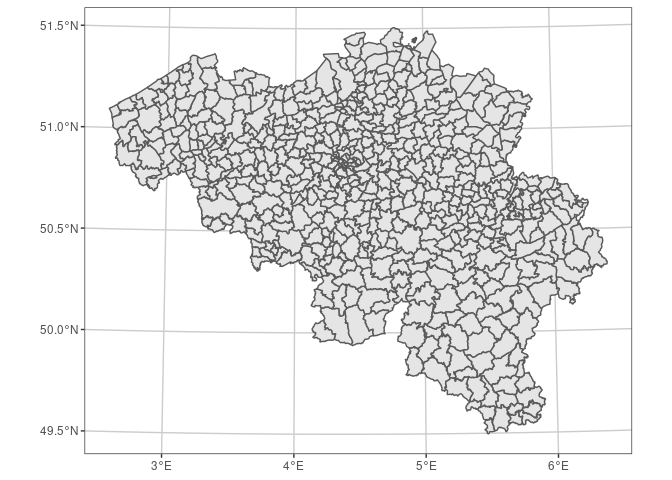
However, mind that the simplification may be OK for mapping at an appropriate scale, but beware that information has been lost, so shapes have changed and gaps + overlaps will appear between polygons. Hence don’t use this simplified version if you process it further, or for detailed mapping.
Note the latitude-longitude graticule: the map follows the CRS of the plotted object, but the graticule is latitude-longitude by default.
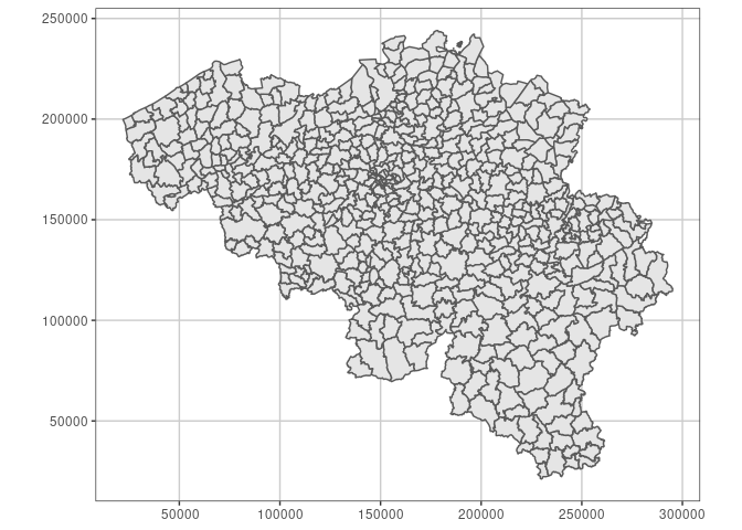
We can plot the graticule of another CRS with coord_sf():
ggplot(data = comm_simpl_31370) + geom_sf() + coord_sf(datum = "EPSG:31370")
The above is the most obvious choice here, since it’s the CRS of the
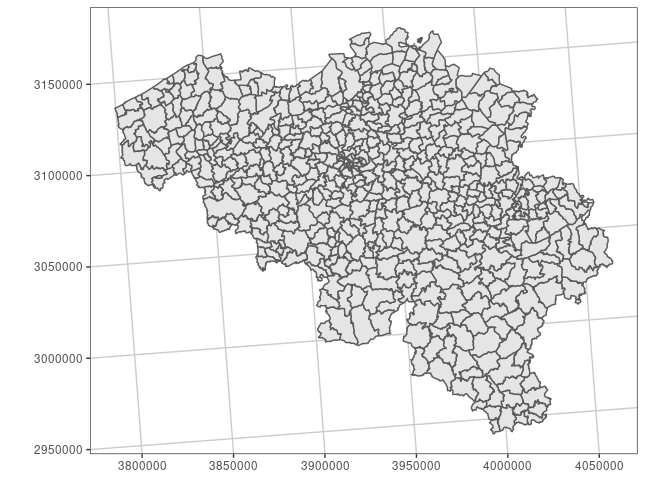
object, but we could as well plot the graticule of e.g. EPSG:3035
(ETRS89-extended / LAEA Europe):
ggplot(data = comm_simpl_31370) + geom_sf() + coord_sf(datum = "EPSG:3035")
Next to the ggplot2 package, which
we used above, interactive maps can be made with the
mapview package.
Here too, time to render differs between:
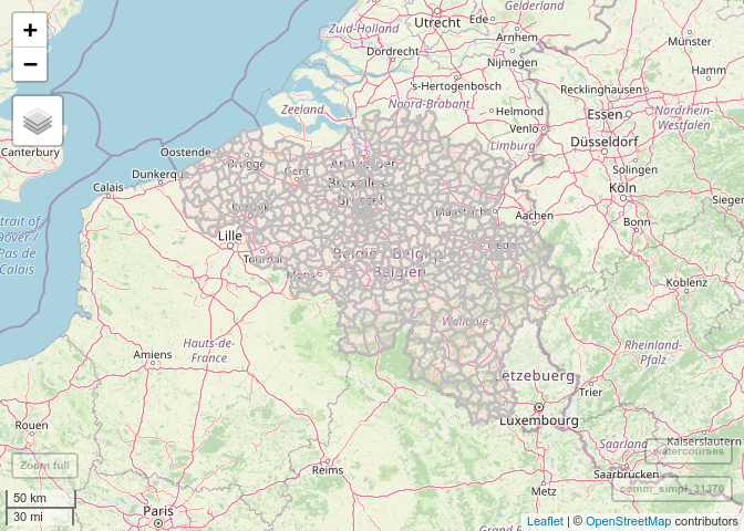
mapview(municipalities_31370, legend = FALSE)
and:
mapview(comm_simpl_31370, legend = FALSE)
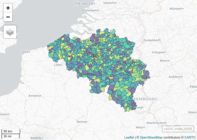
Note: run the code to see this and the following interactive maps.
In this case, mapview is using the leaflet package with some nice
defaults, but in the above examples it makes a color map by default
because there’s only one attribute. We don’t want this and we make some
further adjustments:
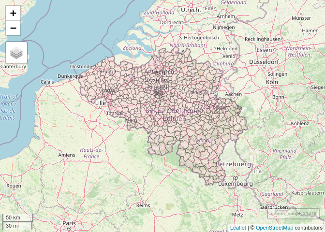
mapview(comm_simpl_31370,
        col.regions = "pink",
        alpha.regions = 0.3,
        legend = FALSE,
        map.types = "OpenStreetMap")
Note that a separate tutorial about leaflet is
available on this website!
Beware that mapview and leaflet produce maps in the ‘WGS 84 /
Pseudo-Mercator’ CRS (EPSG:3857). For that to happen, mapview
transforms spatial objects on-the-fly. Pseudo Mercator or Web
Mercator is a
much used projection in web mapping because the coordinate projection is
computed much faster. However it should not be used in official mapping
or as a projected CRS for geoprocessing, since it has more distortions
(including shape) than e.g. the (truly) conformal Mercator projection
(e.g. in CRS EPSG:3395 – WGS 84 / World Mercator – which is best used
in the equatorial region).
Let’s show two layers with mapview:
mapview(list(comm_simpl_31370, watercourses),
        col.regions = c("pink", "blue"),
        alpha.regions = c(0.2, 0.5),
        color = c("grey", NA),
        legend = FALSE,
        map.types = "OpenStreetMap")
Different transformation pipelines
We consider a layer of points that correspond to locations where characteristics were determined of Flemish surfacewater bodies:
path_points <- file.path(gisclubdata_path, "meetplaatsen_oppwater.shp")
points <- read_sf(path_points)
Check the CRS:
st_crs(points)
Coordinate Reference System:
  User input: Amersfoort / RD New
  wkt:
PROJCRS["Amersfoort / RD New",
    BASEGEOGCRS["Amersfoort",
        DATUM["Amersfoort",
            ELLIPSOID["Bessel 1841",6377397.155,299.1528128,
                LENGTHUNIT["metre",1]]],
        PRIMEM["Greenwich",0,
            ANGLEUNIT["degree",0.0174532925199433]],
        ID["EPSG",4289]],
    CONVERSION["RD New",
        METHOD["Oblique Stereographic",
            ID["EPSG",9809]],
        PARAMETER["Latitude of natural origin",52.1561605555556,
            ANGLEUNIT["degree",0.0174532925199433],
            ID["EPSG",8801]],
        PARAMETER["Longitude of natural origin",5.38763888888889,
            ANGLEUNIT["degree",0.0174532925199433],
            ID["EPSG",8802]],
        PARAMETER["Scale factor at natural origin",0.9999079,
            SCALEUNIT["unity",1],
            ID["EPSG",8805]],
        PARAMETER["False easting",155000,
            LENGTHUNIT["metre",1],
            ID["EPSG",8806]],
        PARAMETER["False northing",463000,
            LENGTHUNIT["metre",1],
            ID["EPSG",8807]]],
    CS[Cartesian,2],
        AXIS["easting (X)",east,
            ORDER[1],
            LENGTHUNIT["metre",1]],
        AXIS["northing (Y)",north,
            ORDER[2],
            LENGTHUNIT["metre",1]],
    USAGE[
        SCOPE["Engineering survey, topographic mapping."],
        AREA["Netherlands - onshore, including Waddenzee, Dutch Wadden Islands and 12-mile offshore coastal zone."],
        BBOX[50.75,3.2,53.7,7.22]],
    ID["EPSG",28992]]
The points object has the projected ‘Amersfoort / RD New’ CRS
(EPSG:28992), which was created for The Netherlands – onshore. See
e.g.
Wikipedia
for more background about this CRS.
Essentially we are dealing with a different projected CRS than
EPSG:31370. EPSG:28992 uses the ‘Amersfoort’ geodetic datum, defined
using the ‘Bessel 1841’ ellipsoid, while EPSG:31370 has the ‘Reseau
National Belge 1972’ datum, defined using the ‘International 1924’
ellipsoid.1
We will transform points (back) to EPSG:31370 since the data are
outside the intended area of usage. Note that this dataset has been made
for mere demonstrative purposes: since at least a part of the points
fall outside the area of usage (geographic bounding box) of the
‘Amersfoort / RD New’ CRS, the dataset is not appropriate to start from.
But let’s suppose it is all one had available to work with!
Standard approach
By default, the appropriate transformation pipeline (concatenated coordinate operations) can differ between different areas that are represented in a spatial dataset. This is taken care of automatically, based on the bounding boxes of each CRS, but it will also depend on the availability of specific transformation grids.
points_31370 <- st_transform(points, "EPSG:31370")
Notice the completely different coordinate ranges between both CRSs:
st_geometry(points)
#> Geometry set for 7320 features
#> Geometry type: POINT
#> Dimension:     XY
#> Bounding box:  xmin: -62470.03 ymin: 300542 xmax: 193543.8 ymax: 427302.7
#> Projected CRS: Amersfoort / RD New
#> First 5 geometries:
#> POINT (-30849.68 354341.7)
#> POINT (-31237.91 354683.3)
#> POINT (-28757.74 356391.3)
#> POINT (709.4341 373861.2)
#> POINT (116680.8 340639.1)
st_geometry(points_31370)
#> Geometry set for 7320 features
#> Geometry type: POINT
#> Dimension:     XY
#> Bounding box:  xmin: 3174.827 ymin: 152992.4 xmax: 260391 ymax: 278347.1
#> Projected CRS: BD72 / Belgian Lambert 72
#> First 5 geometries:
#> POINT (35483.62 205530.5)
#> POINT (35090.55 205866.5)
#> POINT (37545.94 207609.8)
#> POINT (66666.83 225461.1)
#> POINT (183089.2 193870.8)
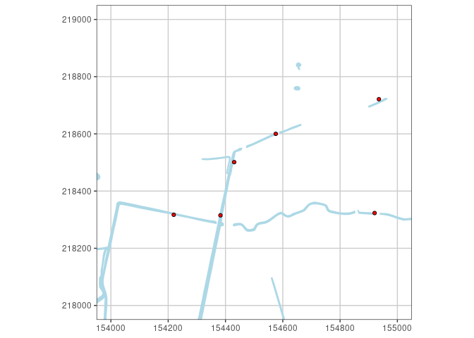
A specific area shown with ggplot2 in EPSG:31370:
ggplot() +
  geom_sf(data = watercourses, fill = "lightblue", colour = "lightblue") +
  geom_sf(data = points_31370, fill = "red", shape = 21) +
  lims(x = c(154e3, 155e3), y = c(218e3, 219e3)) +
  coord_sf(datum = "EPSG:31370")
Enforcing a specific pipeline
We can request available transformation pipelines with
sf_proj_pipelines():
pipelines <- sf_proj_pipelines("EPSG:28992", "EPSG:31370")
One can further limit this by specifying the area of interest (aoi
argument), which we didn’t do here.
It is a dataframe with following structure:
glimpse(pipelines)
Rows: 13
Columns: 9
$ id           <chr> "pipeline", "pipeline", "pipeline", "pipeline", "pipeline…
$ description  <chr> "Inverse of RD New + Amersfoort to ETRS89 (9) + Inverse o…
$ definition   <chr> "+proj=pipeline +step +inv +proj=sterea +lat_0=52.1561605…
$ has_inverse  <lgl> TRUE, TRUE, TRUE, TRUE, TRUE, TRUE, TRUE, TRUE, TRUE, TRU…
$ accuracy     <dbl> 0.011, 0.201, 0.260, 0.450, 1.001, 1.250, 2.000, 2.000, 2…
$ axis_order   <lgl> FALSE, FALSE, FALSE, FALSE, FALSE, FALSE, FALSE, FALSE, F…
$ grid_count   <int> 2, 1, 1, 0, 1, 0, 0, 0, 0, 0, 0, 0, 0
$ instantiable <lgl> TRUE, TRUE, TRUE, TRUE, TRUE, TRUE, TRUE, TRUE, TRUE, TRU…
$ containment  <lgl> FALSE, FALSE, FALSE, FALSE, FALSE, FALSE, FALSE, FALSE, F…
Some metadata about the pipelines:
pipelines %>%
  as_tibble %>%
  select(definition, description, grid_count, accuracy, instantiable)
# A tibble: 13 × 5
   definition             description           grid_count accuracy instantiable
   <chr>                  <chr>                      <int>    <dbl> <lgl>
 1 +proj=pipeline +step … Inverse of RD New + …          2    0.011 TRUE
 2 +proj=pipeline +step … Inverse of RD New + …          1    0.201 TRUE
 3 +proj=pipeline +step … Inverse of RD New + …          1    0.26  TRUE
 4 +proj=pipeline +step … Inverse of RD New + …          0    0.45  TRUE
 5 +proj=pipeline +step … Inverse of RD New + …          1    1.00  TRUE
 6 +proj=pipeline +step … Inverse of RD New + …          0    1.25  TRUE
 7 +proj=pipeline +step … Inverse of RD New + …          0    2     TRUE
 8 +proj=pipeline +step … Inverse of RD New + …          0    2     TRUE
 9 +proj=pipeline +step … Inverse of RD New + …          0    2     TRUE
10 +proj=pipeline +step … Inverse of RD New + …          0    2     TRUE
11 +proj=pipeline +step … Inverse of RD New + …          0    6     TRUE
12 +proj=pipeline +step … Inverse of RD New + …          0    6     TRUE
13 +proj=pipeline +step … Inverse of RD New + …          0   NA     TRUE
We can see that the first one has best accuracy. Several pipelines are based on one or two grids for a better accuracy.
When printing the pipelines object, its first row is printed in a more
readable manner:
pipelines
Candidate coordinate operations found:  13
Strict containment:     FALSE
Axis order auth compl:  FALSE
Source:  EPSG:28992
Target:  EPSG:31370
Best instantiable operation has accuracy: 0.011 m
Description: Inverse of RD New + Amersfoort to ETRS89 (9) + Inverse of BD72
             to ETRS89 (3) + Belgian Lambert 72
Definition:  +proj=pipeline +step +inv +proj=sterea +lat_0=52.1561605555556
             +lon_0=5.38763888888889 +k=0.9999079 +x_0=155000
             +y_0=463000 +ellps=bessel +step +proj=hgridshift
             +grids=nl_nsgi_rdtrans2018.tif +step +inv
             +proj=hgridshift
             +grids=be_ign_bd72lb72_etrs89lb08.tif +step
             +proj=lcc +lat_0=90 +lon_0=4.36748666666667
             +lat_1=51.1666672333333 +lat_2=49.8333339
             +x_0=150000.013 +y_0=5400088.438 +ellps=intl
Since the rows of pipelines are sorted by instantiable and accuracy,
it makes sense to designate the printed pipeline as Best instantiable
operation.
It follows that the same information appears when manually selecting and then printing, except for the number of ‘candidate operations found’:
pipelines[1,]
Candidate coordinate operations found:  1
Strict containment:     FALSE
Axis order auth compl:  FALSE
Source:  EPSG:28992
Target:  EPSG:31370
Best instantiable operation has accuracy: 0.011 m
Description: Inverse of RD New + Amersfoort to ETRS89 (9) + Inverse of BD72
             to ETRS89 (3) + Belgian Lambert 72
Definition:  +proj=pipeline +step +inv +proj=sterea +lat_0=52.1561605555556
             +lon_0=5.38763888888889 +k=0.9999079 +x_0=155000
             +y_0=463000 +ellps=bessel +step +proj=hgridshift
             +grids=nl_nsgi_rdtrans2018.tif +step +inv
             +proj=hgridshift
             +grids=be_ign_bd72lb72_etrs89lb08.tif +step
             +proj=lcc +lat_0=90 +lon_0=4.36748666666667
             +lat_1=51.1666672333333 +lat_2=49.8333339
             +x_0=150000.013 +y_0=5400088.438 +ellps=intl
If you’d like to get even more metadata on the available pipelines,
including the WKT definitions, you can also run PROJ’s
projinfo command line program
from within R if it’s available in your system PATH.
system("projinfo -s EPSG:28992 -t EPSG:31370 --spatial-test intersects -o WKT2:2019")
The default operation returned by PROJ’s projinfo, based on the
union of the source and target CRS’s bounding box, appears to be just
one pipeline with so-called ballpark
accuracy.
It’s obtained by dropping the --spatial-test intersects option (or
replacing intersects by contains, which is default)2, and so it
matches the pipeline where accuracy equals NA in our pipelines
dataframe:
pipelines[13,]
Candidate coordinate operations found:  1
Strict containment:     FALSE
Axis order auth compl:  FALSE
Source:  EPSG:28992
Target:  EPSG:31370
Best instantiable operation has only ballpark accuracy
Description: Inverse of RD New + Ballpark geographic offset from Amersfoort
             to BD72 + Belgian Lambert 72
Definition:  +proj=pipeline +step +inv +proj=sterea +lat_0=52.1561605555556
             +lon_0=5.38763888888889 +k=0.9999079 +x_0=155000
             +y_0=463000 +ellps=bessel +step +proj=lcc
             +lat_0=90 +lon_0=4.36748666666667
             +lat_1=51.1666672333333 +lat_2=49.8333339
             +x_0=150000.013 +y_0=5400088.438 +ellps=intl
The low accuracy of a ballpark transformation is because datum differences between source and target CRSs are neglected:
It does not attempt any datum shift, hence the “ballpark” qualifier in its name. Its accuracy is unknown, and could lead in some cases to errors of a few hundreds of metres.
(Source: https://proj.org/glossary.html#term-Ballpark-transformation)
With st_transform() we can enforce a specific pipeline. Note that it
is only available for sfc objects, not sf objects.
Let’s apply the most accurate pipeline to all points:
# We select the pipeline with lowest accuracy (< 0.02), by filtering on accuracy.
# If the grids are installed, this should match the first line of the pipelines object.
chosen_pipeline_definition <- pipelines %>% filter(accuracy < 0.02) %>% pull(definition)
points_31370_strict <-
  st_transform(st_geometry(points), "EPSG:31370",
               pipeline = chosen_pipeline_definition) %>%
  st_sf(st_drop_geometry(points), geometry = .) %>%
  as_tibble %>%
  st_as_sf
And compare:
st_geometry(points_31370)
#> Geometry set for 7320 features
#> Geometry type: POINT
#> Dimension:     XY
#> Bounding box:  xmin: 3174.827 ymin: 152992.4 xmax: 260391 ymax: 278347.1
#> Projected CRS: BD72 / Belgian Lambert 72
#> First 5 geometries:
#> POINT (35483.62 205530.5)
#> POINT (35090.55 205866.5)
#> POINT (37545.94 207609.8)
#> POINT (66666.83 225461.1)
#> POINT (183089.2 193870.8)
st_geometry(points_31370_strict)
#> Geometry set for 7320 features  (with 9 geometries empty)
#> Geometry type: POINT
#> Dimension:     XY
#> Bounding box:  xmin: 18976.03 ymin: 152963.3 xmax: 260391 ymax: 244024
#> Projected CRS: BD72 / Belgian Lambert 72
#> First 5 geometries:
#> POINT (35393.39 205495.3)
#> POINT (35000.39 205831.3)
#> POINT (37455.41 207574.3)
#> POINT (66666.83 225461.1)
#> POINT (183089.2 193870.8)
Notice the 9 empty geometries in case of points_31370_strict!
What is happening?
p <-
  ggplot() +
  geom_sf(data = points_31370, colour = "red") +
  geom_sf(data = points_31370_strict, colour = "green")
p
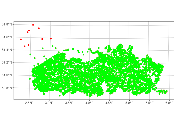
It appears that points too far at sea are considered invalid when applying this pipeline, and their geometry was cleared (although the corresponding row was not dropped).
If we make a zoomable plot, there’s more to discover.
plotly::ggplotly(p)
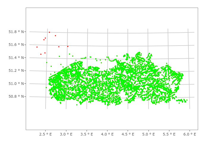
Most points on the map are on the exact same location between both approaches. We can see that points west and south of the geographic bounding box for usage of the Dutch CRS have a different position depending on the applied approach.
It can be further investigated with mapview (note that this does a
further reprojection to EPSG:3857):
mapview(list(points_31370, points_31370_strict),
        col.regions = c("red", "green"))
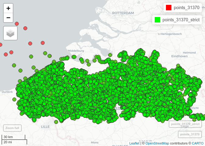
Here it appears that the western and southern points of points_31370
were transformed with the ballpark-accuracy pipeline: they are way off
the surfacewater bodies!
In this case, one might prefer enforcing the specific pipeline outside
the geographic bounding box of EPSG:28992, as we did for
points_31370_strict. However best explore the other pipelines as well,
e.g. the most accurate one that doesn’t depend on a grid, and consider
using that outside the geographic bounding box.
Bottomline is that you should be suspicious about coordinates outside the CRS’s geographic bounding box! So keep an eye on them when applying a default transformation procedure.
Further reading and more packages
Much more information can be found in the online books by Pebesma &
Bivand (2021)
and Lovelace et al.
(2019). The sf package has a nice
website at https://r-spatial.github.io/sf; version 0.6-1 was
introduced in Pebesma
(2018).
There are several more R packages to make beautiful maps. We
specifically mention tmap
(Tennekes, 2018) and
mapsf for making production-ready
thematic maps. tmap is used a lot in Lovelace et
al.
(2019).
Further, there is the
plotKML package, which
renders spatial objects in Google Earth (Hengl et al.,
2015)!
Bibliography
Hengl T., Roudier P., Beaudette D. & Pebesma E. (2015). plotKML: Scientific Visualization of Spatio-Temporal Data. Journal of Statistical Software 63. http://www.geostat-course.org/system/files/jss1079.pdf.
Lovelace R., Nowosad J. & Muenchow J. (2019). Geocomputation with R. https://geocompr.robinlovelace.net/.
Pebesma E. (2018). Simple Features for R: Standardized Support for Spatial Vector Data. The R Journal 10 (1): 439–446. https://journal.r-project.org/archive/2018/RJ-2018-009/index.html.
Pebesma E. & Bivand R. (2021). Spatial Data Science. https://r-spatial.org/book.
Tennekes M. (2018). tmap: Thematic Maps in R. Journal of Statistical Software 84 (1): 1–39. https://doi.org/10.18637/jss.v084.i06.
-
Note that several European countries, including Belgium, now provide national projected CRSs that use the common ETRS89 datum (European Terrestrial Reference System 1989). An example is the Belgian CRS
EPSG:3812(ETRS89 / Belgian Lambert 2008). ↩︎ -
In the documentation of
projinfo, we can read about the--spatial-testoption: ‘Specify how the area of use of coordinate operations found in the database are compared to the area of use specified explicitly with--areaor--bbox, or derived implicitly from the area of use of the source and target CRS. By default, projinfo will only keep coordinate operations whose area of use is strictly within the area of interest (contains strategy). If using the intersects strategy, the spatial test is relaxed, and any coordinate operation whose area of use at least partly intersects the area of interest is listed.’ ↩︎