Same variable in fixed and random effects • Thierry Onkelinx

Used packages

library(ggplot2)

## Warning: package 'ggplot2' was built under R version 4.0.2

library(lme4)

## Loading required package: Matrix

Dummy data

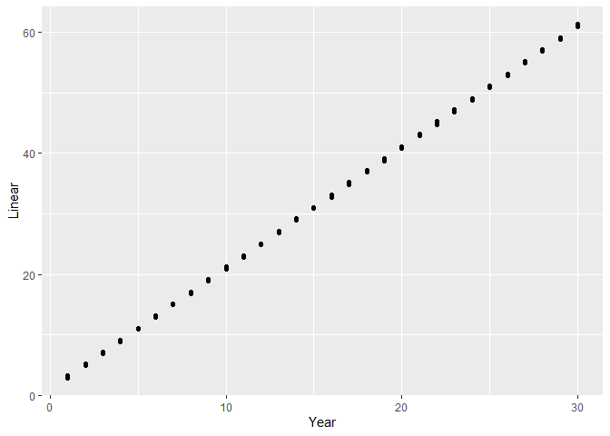
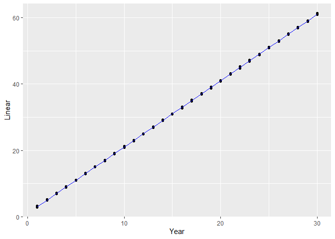
For the sake of this demontration we use a very simple dataset with a very high signal versus noise ratio. Let’s look at a simple timeseries with multiple observations per timepoint.

set.seed(213354)
n.year <- 30
n.replicate <- 10
sd.noise <- 0.1
dataset <- expand.grid(
  Replicate =  seq_len(n.replicate),
  Year = seq_len(n.year)
)
dataset$fYear <- factor(dataset$Year)
dataset$Noise <- rnorm(nrow(dataset), mean = 0, sd = sd.noise)
dataset$Linear <- 1 + 2 * dataset$Year + dataset$Noise
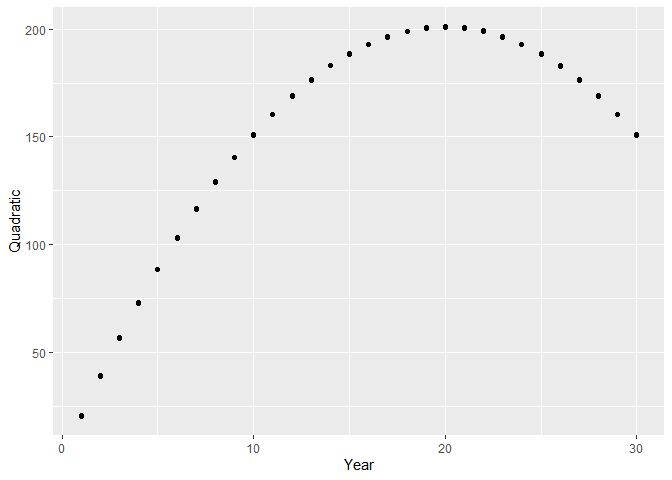
dataset$Quadratic <- 1 + 20 * dataset$Year - 0.5 * dataset$Year ^ 2 + 
  dataset$Noise

ggplot(dataset, aes(x = Year, y = Linear)) + geom_point()

ggplot(dataset, aes(x = Year, y = Quadratic)) + geom_point()

Quadratic trend but fit as a linear trend

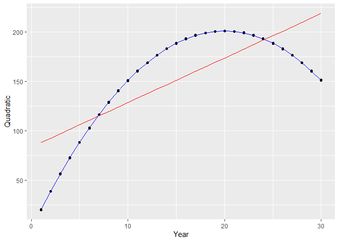
Assume that we assume that the trend is linear but in reality it is quadratic. In this case the random intercept of year will pickup the differences with the linear trend.

model.quadratric <- lmer(Quadratic ~ Year + (1|Year), 
                         data = dataset)
summary(model.quadratric)

## Linear mixed model fit by REML ['lmerMod']
## Formula: Quadratic ~ Year + (1 | Year)
##    Data: dataset
## 
## REML criterion at convergence: -90.8
## 
## Scaled residuals: 
##      Min       1Q   Median       3Q      Max 
## -2.13929 -0.65021 -0.00099  0.55503  3.14673 
## 
## Random effects:
##  Groups   Name        Variance  Std.Dev.
##  Year     (Intercept) 1198.1591 34.6144 
##  Residual                0.0111  0.1054 
## Number of obs: 300, groups:  Year, 30
## 
## Fixed effects:
##             Estimate Std. Error t value
## (Intercept)  83.6622    12.9622   6.454
## Year          4.4999     0.7301   6.163
## 
## Correlation of Fixed Effects:
##      (Intr)
## Year -0.873

dataset$QuadraticPredict <- predict(model.quadratric)
dataset$QuadraticFixed <- predict(model.quadratric, re.form = ~0)

ggplot(dataset, aes(x = Year, y = Quadratic)) + 
  geom_point() + 
  geom_line(aes(y = QuadraticFixed), colour = "red") + 
  geom_line(aes(y = QuadraticPredict), colour = "blue")

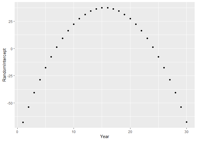
The random effects will have a strong pattern. Indicating that a second order polynomial makes more sense than a linear trend.

rf <- data.frame(
  Year = seq_len(n.year),
  RandomIntercept = ranef(model.quadratric)$Year[, 1]
)

ggplot(rf, aes(x = Year, y = RandomIntercept)) + 
  geom_point()

What if the trend is perfectly linear?

Both the fixed effect and the random effect can perfectly model the pattern in the data. So the model seems to be unidentifiable. However the likelihood of the model contains a penalty term for the random intercept. The stronger the absolute value of the random effect, the stronger the penalty. The fixed effects have no penalty term. Hence, model with strong fixed effect will have a higher likelihood than exactly the same fit generated by strong random effects.

In this case the linear trend is very strong compared to the noise. So the linear trend in the fixed effect fits the data very well. Note that the random effect variance is zero.

model.linear <- lmer(Linear ~ Year + (1|Year), data = dataset)

## boundary (singular) fit: see ?isSingular

summary(model.linear)

## Linear mixed model fit by REML ['lmerMod']
## Formula: Linear ~ Year + (1 | Year)
##    Data: dataset
## 
## REML criterion at convergence: -483.9
## 
## Scaled residuals: 
##     Min      1Q  Median      3Q     Max 
## -2.3565 -0.6669 -0.0309  0.5717  3.0381 
## 
## Random effects:
##  Groups   Name        Variance Std.Dev.
##  Year     (Intercept) 0.00000  0.0000  
##  Residual             0.01095  0.1046  
## Number of obs: 300, groups:  Year, 30
## 
## Fixed effects:
##             Estimate Std. Error t value
## (Intercept) 0.995497   0.012392   80.34
## Year        1.999948   0.000698 2865.22
## 
## Correlation of Fixed Effects:
##      (Intr)
## Year -0.873
## convergence code: 0
## boundary (singular) fit: see ?isSingular

dataset$LinearPredict <- predict(model.linear)
dataset$LinearFixed <- predict(model.linear, re.form = ~0)

ggplot(dataset, aes(x = Year, y = Linear)) + 
  geom_point() + 
  geom_line(aes(y = LinearFixed), colour = "red") + 
  geom_line(aes(y = LinearPredict), colour = "blue")

What about fitting year as a factor in the fixed effects

Combining the same variables as a factor in the fixed effects and as a random intercept doesn’t make sense. They allow exactly the same model fit and thus the random intercept will always shrink to zero.