Darwin Core mapping
Lien Reyserhove
Peter Desmet
2018-02-26
1 Introduction
This tutorial describes how to standardize or map data to Darwin Core using R. We’ll mainly use functions from the dplyr package (see our introduction to dplyr). We recommend using a step-by-step approach mapping data to Darwin Core:
1. Setup
  - Load libraries
  - Define locale
2. Import and clean data
  - Import data
  - Inspect data
  - Clean data
3. Map to Darwin Core Archive
  - Pre-processing
  - Mapping
  - Post-processing
We’ll walk through the tutorial step-by-step by using the Inventory of alien macroinvertebrates in Flanders, Belgium as an example.
2 Setup
We load the libraries necessary to import, clean and map the data:
library(tidyverse) # For data transformation (includes dplyr)
library(magrittr)  # For %<>% pipes
library(readxl)    # For reading excel files
library(janitor)   # For basic cleaning of the data
Before we load the data, we define the locale:
Sys.setlocale("LC_CTYPE", "en_US.UTF-8")## [1] "en_US.UTF-8"3 Import and clean data
3.1 Import data
Our raw datasat is an Excel file (AI_2016_Boets_etal_Supplement.xls). The import specifications for Excel files are more limited than those for delimited files (csv, tsv, txt). However, we think it’s useful to use Excel as a format in this exercise as this is often used to manage datasets.
- Go to
Environmentpanel:Import dataset > From Excel... - For
File/URL, clickBrowseand selectAI_2016_Boets_etal_Supplement.xls - Specify the
Import Options:Name:raw_dataSheet:checklistNA:NAor leave emptyFirst Row as Names: check
- Click on
Data previewto verify if everything looks OK - Click
Importto generate the dataframe
3.2 Inspect data
The simplest way for a quick overview of the raw data is by using the functions str() and head():
str(raw_data) ## Classes 'tbl_df', 'tbl' and 'data.frame': 73 obs. of 12 variables:
## $ Taxon ID : chr "SAGAEFWEV" "SFGSTHSIM" "XIGXULXGI" "ZVJOBJJJX" ...
## $ Phylum : chr "Crustacea" "Crustacea" "Crustacea" "Crustacea" ...
## $ Order : chr "Sessilia" "Sessilia" "Sessilia" "Decapoda" ...
## $ Family : chr "Balanidae" "Balanidae" "Balanidae" "Astacidae" ...
## $ Species : chr "Amphibalanus amphitrite" "Amphibalanus improvisus" "Amphibalanus reticulatus" "Astacus leptodactylus" ...
## $ Origin : chr "South-Europe" "West-Atlantic" "Tropical and warm seas" "East-Europe" ...
## $ First occurrence in Flanders: chr "1952" "before 1700" "1997" "1986" ...
## $ Pathway of introduction : chr "shipping" "shipping" "shipping" "aquaculture" ...
## $ Pathway mapping : chr "Ship/boat hull fouling" "Ship/boat hull fouling | Ship/boat ballast water | Contaminant on animals (except parasites, species transporte"| __truncated__ "Ship/boat hull fouling" "Aquaculture | Pet/aquarium/terrarium species (including live food for such species )" ...
## $ Salinity zone : chr "M" "M" "M" "F" ...
## $ Reference : chr "Kerckhof and Catrijsse 2001" "Kerckhof and Catrijsse 2001" "Kerckhof and Catrijsse 2001" "Gerard 1986" ...
## $ Pathway mapping remarks : chr NA "considered transport with oyster lots as 'Contaminant on animals'" NA NA ...head(raw_data) # Displays the first 6 lines of the dataframe3.3 Clean data
We assume here that your dataset is tidy. If this is not the case, we refer to the [Tidy data exercise]. Unfortunately, starting with untidy data will make your script a lot more complex, with many preparatory steps before you can even start mapping! In a tidy dataset, you can start the mapping immediately.
In some cases, some small cleaning steps could be made to clean raw_data. Here, the column names of raw_data contain capital letters:
colnames(raw_data)## [1] "Taxon ID" "Phylum"
## [3] "Order" "Family"
## [5] "Species" "Origin"
## [7] "First occurrence in Flanders" "Pathway of introduction"
## [9] "Pathway mapping" "Salinity zone"
## [11] "Reference" "Pathway mapping remarks"It’s easier to use lower case letters only and to discard all spaces in the column names. The package janitor provides some useful tools for this:
raw_data %<>% clean_names() ## [1] "taxon_id" "phylum"
## [3] "order" "family"
## [5] "species" "origin"
## [7] "first_occurrence_in_flanders" "pathway_of_introduction"
## [9] "pathway_mapping" "salinity_zone"
## [11] "reference" "pathway_mapping_remarks"During the mapping, we will sequentially add new Darwin Core terms (see further). To avoid name clashes between the original columns in raw_data and the added Darwin Core columns, we add the prefix raw_ to the column names of raw_data:
# Add prefix `raw_` to the column names of `raw_data`.
colnames(raw_data) <- paste0("raw_", colnames(raw_data))
## [1] "raw_taxon_id" "raw_phylum"
## [3] "raw_order" "raw_family"
## [5] "raw_species" "raw_origin"
## [7] "raw_first_occurrence_in_flanders" "raw_pathway_of_introduction"
## [9] "raw_pathway_mapping" "raw_salinity_zone"
## [11] "raw_reference" "raw_pathway_mapping_remarks"We’re now all set to start mapping!
4 Map to Darwin Core Archive
Even though raw_data contains all necessary information in a single data frame, a Darwin Core Archive might consist of multiple files, e.g. a core and extensions. We recommend to create the core file first and then the extensions. For each file, there are 3 steps:
- Pre-processing step: basic preparations before the mapping
- Mapping: sequential addition of the Darwin Core fields based on the raw values
- Post-processing step: removing the raw values and saving the file
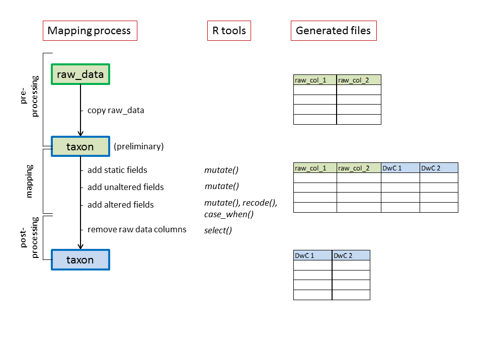
Schematic overview of the mapping process
This is repeated for each core/extension file. Below, we’ll use the taxon core as an example.
4.1 Pre-processing
We use a copy of raw_data as the starting point for the mapping of the taxon core. This is because raw_data is the starting point for the mapping of both the taxon core and the extensions. It needs to be untouched each time we start the mapping process.
taxon <- raw_data # Generate taxon by making a copy of raw_dataSometimes there are further pre-processing steps needed. E.g. in a vernacular name extension each name is a row, while in the original data the names could be columns or delimited values within a column. That kind of data requires separate() en gather() steps first. Here however, each record is taxon and no further pre-processing steps are required.
4.2 Mapping
The mapping process is sequential: we add the Darwin Core terms to taxon step by step. The Darwin Core terms for each core/extension file can be found on the GBIF Resources page:
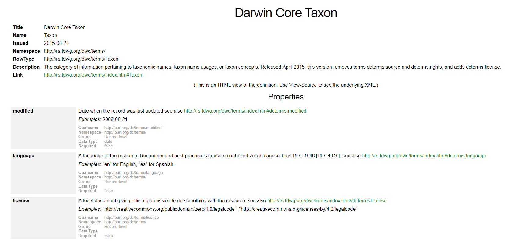
It is good practice to inspect the Darwin Core terms on this webpage one by one to see whether a particular term can be used in your checklist. We respect the order of the terms as they listed on the GBIF resource page.
We distinguish three types of Darwin Core terms mappings (static values, unaltered values and altered values) and for each one we will use mutate() and %<>% (double pipe).
4.2.1 Static values
Static values are used for Darwin Core terms that need the same value for all records. Most often, they are absent in raw_data. This mostly concerns metadata fields in the taxon core file:
taxon %<>% mutate(language = "en")taxon %<>% mutate(license = "http://creativecommons.org/publicdomain/zero/1.0/")taxon %<>% mutate(rightsHolder = "Ghent University Aquatic Ecology")taxon %<>% mutate(datasetID = "https://doi.org/10.15468/yxcq07")taxon %<>% mutate(datasetName = "Inventory of alien macroinvertebrates in Flanders, Belgium")Other, non-metadata fields:
taxon %<>% mutate(kingdom = "Animalia")taxon %<>% mutate(nomenclaturalCode = "ICZN")All these fields are added as extra columns to the data frame, in the same order as they were added:
4.2.2 Unaltered values
Unaltered values are used for Darwin Core terms for which the content is an exact copy of the corresponding field in raw_data. This contrasts with altered fields, in which use a certain field in raw_data is the basis for further processing.
Before deciding whether or not some basic processing is required, it is useful to screen the variables in raw_data for their specific content. distinct() is a useful function to show the unique values for a field:
taxon %>% distinct(raw_phylum)Note
We use %>% instead of %<>%, as we don’t want to add a new column to taxon.
Some unaltered fields:
taxon %<>% mutate(taxonID = raw_taxon_id)taxon %<>% mutate(scientificName = raw_species)taxon %<>% mutate(family = raw_family)View those 3 fields:
4.2.3 Altered values
Altered values are used for Darwin Core terms for which the content in raw_data is used as a basis, but it needs to be standardized. This applies to Darwin Core terms for which we use a vocabulary or where we want to transform for clarity or to correct obvious mistakes.
The main functions we use for these are: mutate() + recode() or mutate() + case_when().
4.2.3.1 mutate() + recode()
In this case, we aim to replace specific information in raw_data by new information specified in the code. For instance, raw_order will be mapped to the Darwin Core term order:
taxon %>% distinct(raw_order)Veneroida is a typo. We need to replace this by Venerida:
taxon %<>%
  mutate(order = recode(raw_order, "Veneroidea" = "Venerida"))
We use select(), group_by_all() and summarize()to compare our newly mapped data with the original data. Note that the other values remain unaltered:
taxon %>%
  select(raw_order, order) %>%
  group_by_all() %>%
  summarize()
Another use case:
raw_phylum will be mapped to to Darwin Core term phylum.
taxon %>% distinct(raw_phylum)However, Crustacea is not a phylum but a subphylum. The phylum to which crustaceans belong is Arthropoda. We can correct this with recode():
taxon %<>% mutate (phylum = recode(raw_phylum, "Crustacea" = "Arthropoda"))Other use cases (not applicable to our data):
distribution %<>% mutate(description = recode(raw_d_n,
  "Ext.?"     = "Ext.",
  "Ext./Cas." = "Cas.",
  "Cas.?"     = "Cas.",
  "Nat.?"     = "Nat.",
  .missing = ""))

distribution %<>% mutate(locality = recode(value,
  "AF"     = "Africa (WGSRPD:2)",
  "AM"     = "pan-American",
  "AS"     = "Asia",
  "AS-Te"  = "temperate Asia (WGSRPD:3)",
  "AS-Tr"  = "tropical Asia (WGSRPD:4)",
  "AUS"    = "Australasia (WGSRPD:5)",
  "Cult."  = "cultivated origin",
  "E"      = "Europe (WGSRPD:1)",
  "Hybr."  = "hybrid origin",
  "NAM"    = "Northern America (WGSRPD:7)",
  "SAM"    = "Southern America (WGSRPD:8)",
  "Trop."  = "Pantropical",
  .default = "",
  .missing = ""
))
4.2.3.2 mutate() + case_when()
case_when is often used together with mutate() when you want to make a new column (or change an existing one) based on the content of other existing variables.
For instance, taxonRank information is lacking in raw_data. We need to generate this information based on the information contained in raw_species:
Inspect raw_species:
taxon %>% distinct(raw_species)Although most raw_species are in fact species, Dreissena rostriformis bugensis is not a species but a subspecies. We need to make this distinction in the mapping process:
taxon %<>% mutate(taxonRank = case_when(
  raw_species == "Dreissena rostriformis bugensis" ~ "subspecies",
  raw_species != "Dreissena rostriformis bugensis" ~ "species")
)
We use select(), group_by_all() and summarize()to compare our newly mapped data with the original data:
taxon %>% select(raw_species, taxonRank) %>%
  group_by_all() %>%
  summarize()
Other use cases (not applicable to our data):
invasion_stage %<>% mutate(description = case_when(
  raw_status == "A" ~ "casual",
  raw_status == "A*" ~ "casual",
  raw_status == "N" ~ "established"
))

distribution %<>%
  mutate(Flanders = case_when(
    raw_presence_fl == "X" & (is.na(raw_presence_br) | raw_presence_br == "?") & (is.na(raw_presence_wa) | raw_presence_wa == "?") ~ "S",
    raw_presence_fl == "?" ~ "?",
    is.na(raw_presence_fl) ~ "NA",
    TRUE ~ "M")) %>%
  mutate(Brussels = case_when(
    (is.na(raw_presence_fl) | raw_presence_fl == "?") & raw_presence_br == "X" & (is.na(raw_presence_wa) | raw_presence_wa == "?") ~ "S",
    raw_presence_br == "?" ~ "?",
    is.na(raw_presence_br) ~ "NA",
    TRUE ~ "M")) %>%
  mutate(Wallonia = case_when(
    (is.na(raw_presence_fl) | raw_presence_fl == "?") & (is.na(raw_presence_br) | raw_presence_br == "?") & raw_presence_wa == "X" ~ "S",
    raw_presence_wa == "?" ~ "?",
    is.na(raw_presence_wa) ~ "NA",
    TRUE ~ "M")) %>%
  mutate(Belgium = case_when(
    raw_presence_fl == "X" | raw_presence_br == "X" | raw_presence_wa == "X" ~ "S", # One is "X"
    raw_presence_fl == "?" | raw_presence_br == "?" | raw_presence_wa == "?" ~ "?" # One is "?"
  ))
4.3 Post-processing
When all terms have been mapped, we remove the raw columns from taxon in order to retain the mapped Darwin Core terms only:
taxon %<>% select(-starts_with("raw_"))Inspect taxon:
head(taxon)As indicated before, it is good practise to keep the order of the Darwin Core fields as specified on the GBIF Resources web page. The mapping process will be a mixture of mapping static fields, unaltered and altered fields.
Save taxon as a csv file. For this, we need to define the path to the taxon core file (relative to this script):
dwc_taxon_file = "../data/processed/taxon.csv"Write as a csv:
write.csv(taxon, file = dwc_taxon_file, na = "", row.names = FALSE, fileEncoding = "UTF-8")Note
Make sure to set na = "" and row.names = FALSE when writing to a CSV file.
5 Exercise
You now know the basics to try yourself!