dplyr
Damiano Oldoni
Stijn Van Hoey
Lien Reyserhove
Peter Desmet
2018-02-26
1 Introduction
This tutorial will provide you the know-how for importing and analysing (tidy) data. We will use the same dataframe to test the most typical dplyr functionalities. There is no better way to improve your programming skills than trying it yourself. Don’t be shy to make faults and take a look to the base R cheatsheet and the dplyr cheatsheet: we do it constantly.
First of all, we need to load some libraries which are part of the tidyverse ecosystem:
library(readr)
library(dplyr)
library(tidyr)
Alternatively, you can load all tidyverse libraries at once by:
library(tidyverse)2 Read data
First of all, we need to import data in R. The most user friendly way to do it is by using the interface provided by RStudio. In the Environment window, click on Import Dataset and select From Text (readr).... A window will pop-up. Follow the next steps:
- Click on
Browseto selet the text file you want to import - Select the right delimiter
- Check whether the class of the column values fits your purpose and in case apply changes by clicking on the class name below the column name
- Change the name in
code previewif you prefer to save the data with a different name than filename - Click on
Import
A dataframe is automatically generated and, very handy, the code to generate it as well! We suggest to use this graphic interface at the beginning in order to be familiar with the most typical parameters (e.g. sep, col_types, col_names, row_names). After a while you will find that writing the code is way faster than a long series of mouse clicks.
2.1 Exercises
- Read
survey_data_spreadsheet_tidy.csv. Check whether the columns match the following types:date:doublespecies:characterplot:integersex:characterweight_in_g:integerdevice_remarks:character
- Save the data into
data:
3 Explore data
Before to start manipulate data, it is best practice exploring the imported dataframe in order to check whether everything is corectly imported and to have an idea about the data we are going to analyse/manipulate. R gives us several tools to do it, which you can test immediately by using one of the many dataframes from the R Datasets package, automatically loaded when you open R. We will use the CO2 dataframe about the carbon dioxide uptake in grass plant Echinochloa crus-galli (details can be found here)
head(CO2)returns the first part of a data frame. It works with several other data types (vectors, tables, …). Specifiy how many rows to display with parametern:haed(CO2, n = ), defaultn = 6view(CO2)opens the entire dataframe in viewer. If dataframe is very big, then your computer can slow down sensibly and Rstudio can eventually crash. Be aware of it!class(CO2)ifCO2is a dataframe then"data.frame"will show upstr(CO2)displays the internal structure of the dataframecol_names(CO2)display column namesnrow(CO2)returns the number of rows of the dataframencol(CO2)return the number of rows of the dataframe
3.1 Exercises
Test the functions introduced above to our dataframe data. In particular:
Display column names:
How many columns are there?
How many rows are there?
Display the first 10 records:
Display data in viewer:
Display structure of data:
4 Sort data
It is normally useful to sort data. The package dplyr offers the function arrange() to do it:
arrange(CO2, conc, uptake)Use parameter desc(col_name) to sort in descending order:
arrange(CO2, desc(conc), desc(uptake))4.1 Exercises
Sort by
datein ascending order:Overwrite
datawith sorted output:
5 Select columns and rows
You can select specific columns of a dataframe by select(). Only columns where conditions are true are selected. For example, selecting a column by its column name:
select(CO2, uptake)To select all columns except a specific column use the minus symbol before its name:
select(CO2, -uptake)To select rows use filter(). Again, one or multiple filters can be applied to filter the targeted rows:
filter(CO2,
  Type == "Quebec",
  Treatment == "nonchilled",
  conc  < 200
)
A condition can be any logical operator (>, >, <=,…). For example, to get only those rows for which the weight_in_g is smaller than 40, use filter(data, weight_in_g < 40).
5.1 Exercises
Display the column
weight_in_g:Display only the records with
weight_in_g > 30:Select females with
weight_in_g > 30:Display only
weight_in_gof females withweight_in_g > 30:Save output of (4) as
females_weight_above_30:Select all columns from
dataexcept thedevice_remarkscolumn:
6 Pipes
As you probably noticed, we need to create new data.frame everytime we want to apply two or more functions. This method has several disadvantages, i.a. messy workspace, higher chance of typos,…
An alternative is to wrap (nest) functions one within each other, so that the output of a function would be considered the input of the other one. For example, if we have to apply f1 to a dataframe df and f2 to the output of f1, we write:
f2(f1(df, ...), ...)filter(select(CO2, uptake), uptake > 30, uptake < 31.8)This way of working with functions is typical of programming and is implemented in many other programming languages. The disadvantage of this approach is readibility: you have to read from right to left in order to understand what happens with our data!
Can we avoid deciphering nested function calls, and making excessive use of temporary data.frames? The answer is yes, thanks to pipe operators. The most used one is the forward pipe: %>%, from the magrittr package. We can then rewrite the example above by using %>%:
df %>% f1(...) %>% f2(...)CO2 %>%
select(uptake) %>%
filter(uptake > 30, uptake < 31.8)Easy, isn’t?
As Stefan Milton, author of magrittr, wrote in this blogpost:
The order in which you’d think of these steps is the same as the order in which they are written, and as the order in which they are executed.
If you want to create a new object (i.e. data.frame) based on the output of a series of functions:
df2 <- df %>% f1(...) %>% f2(...)small_uptakes <- CO2 %>%
select(uptake) %>%
filter(uptake > 30, uptake < 31.8)If you want to overwrite the input dataframe, you can use the compound assignment operator, %<>% which can be read as the composition of the forward pipe %>%, and asignment symbol <-:
df %<>% f1(...) %>% f2(...)We apply all steps on the right of %<>% to df and overwrite it with the final ouput.
library(magrittr)
small_uptakes %<>% filter(uptake < 31)small_uptakesNote
%<>% is part of the package magrittr, which is not loaded with tidyverse or dplyr. You need to load it separately: library(margrittr)
6.1 Exercises
Display the column
weight_in_gwith values > 30 using pipes:Select females with
weight_in_g > 30using pipesDisplay only weight_in_g of females with weight in g > 30:
Save output of (3) as a new
data.frame:females_weight_above_30:
7 Distinct values
The function distinct() retains only unique/distinct values of an input vector. If applied to dataframe, it retains only unique/distinct rows. For example, to know which types of plants were used:
CO2 %>%
  select(Type) %>%
  distinct()
7.1 Exercises
Show the unique sex values:
Show the unique species values:
8 Summarize data
By using select() you can for example calculate minimum or maximum of a specific column.
The minimum uptake:
CO2 %>%
  select(uptake) %>%
  min()
## [1] 7.7And the maximum uptake:
CO2 %>%
  select(uptake) %>%
  max()
## [1] 45.5But what if you want to calculate the minimum and maximum uptake for each plant? You need then to split the data by Plant values and calculate the mimnimum and maximum for each group. We can do it via %>% and two functions from dplyr library: group_by() and summarize():
CO2 %>%
  group_by(Plant) %>%
  summarize(
    min_uptake = min(uptake),
    max_uptake = max(uptake)
  )
Theoretically this kind of workflow is called the split-apply-combine paradigm: split the data into groups, apply some analysis to each group, and then combine the results together.Interesting to notice that group_by actually doesn’t modify the data contained in the dataframe, but adds an internal grouping to the dataframe, which is visible if you run:
class(CO2 %>% group_by(Plant))## [1] "grouped_df" "tbl_df" "tbl" "data.frame"For counting how many rows (with unique) in each group you can use count() instead of summarize():
CO2 %>%
  group_by(Plant) %>%
  count()
8.1 Exercises
Count records per sex:
What is the mean weight? Consider to use function
mean()combined with parameterna.rm = TRUEin order to ignore (remove)NAwhile calculating the mean:Show mean weight per sex:
Show mean weight per sex and species:
Show minimum, maximum and mean weight per sex and species and save output as
weight_per_species_sex. Consider to usemin()andmax()) combined with parameterna.rm = TRUEin order to ignoreNAwhile calculating minimum and maximum:
9 Reshape data
These two functions provide opposite functionalities. While spread() spreads rows into columns, gather() gathers columns into rows. An example can be found in these two images from Data Carpentry:
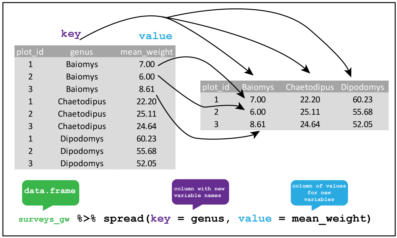
spread

gather
Notice that spread() and gather() aren’t dplyr functions but come from the tidyr library.
9.1 Exercises
Spread
weight_per_species_sexto key onsexand values frommean_weightand save output asweight_per_species_sex_spread:Gather back the data and save output as
weight_per_species_sex_gather. Isweight_per_species_sex_gatherequal toweight_per_species_sex?
10 Rename, add and update columns
Sometimes you need to rename one or more columns. You can do it using function rename():
df %>% rename(new_colname = old_colname)An example:
CO2 %>% rename(Conc = conc)Another typical data analysis task is to create new columns based on the values of existing ones, like converting units or calculating the ratio of values in two columns. We can use the function mutate():
new_df <- df %>% mutate(new_column = ...)An example using CO2 dataframe:
CO2_dev_mean <- CO2 %>% mutate(dev_mean_uptake = uptake - mean(uptake))Or you can modify the original dataframe:
df %<>% mutate(new_column = ...)CO2 %<>% mutate(dev_mean_uptake = uptake - mean(uptake))
head(CO2)You can also use mutate() to change the values in a column without creating a new one. In the example below we change the new column dev_mean_uptake by applying absolute value:
CO2 %<>% mutate(dev_mean_uptake = abs(dev_mean_uptake))

head(CO2)
10.1 Exercises
Rename column
weight_in_gofdatatoweightand overwritedata:Convert
weightvalues in gram to kg:Add column
countrywith a fixed valueUS:Add column
parsed_dateby applying the functionas.Date(column)to thedatecolumn:
11 Translate data
Have you ever wanted to use a kind of find and replace function in R? Then it’s time to use the dplyr functions recode() and case_when: the first function allows you to replace specific values based on a logical condition and it works with vectors. An example:
types <- CO2$Type # Extract Type from dataframe

recode(types,
  Quebec = "Canada",
  Mississippi = "USA"
)
## [1] Canada Canada Canada Canada Canada Canada Canada Canada Canada Canada
## [11] Canada Canada Canada Canada Canada Canada Canada Canada Canada Canada
## [21] Canada Canada Canada Canada Canada Canada Canada Canada Canada Canada
## [31] Canada Canada Canada Canada Canada Canada Canada Canada Canada Canada
## [41] Canada Canada USA USA USA USA USA USA USA USA
## [51] USA USA USA USA USA USA USA USA USA USA
## [61] USA USA USA USA USA USA USA USA USA USA
## [71] USA USA USA USA USA USA USA USA USA USA
## [81] USA USA USA USA
## Levels: Canada USAYou can specify a default value: it will be given to all values not otherwise matched. And if you want replace missing values (NA), then you can specify a value to the parameter missing.
recode(types,
  Quebec = "Canada",
  .default = "World"
)
## [1] Canada Canada Canada Canada Canada Canada Canada Canada Canada Canada
## [11] Canada Canada Canada Canada Canada Canada Canada Canada Canada Canada
## [21] Canada Canada Canada Canada Canada Canada Canada Canada Canada Canada
## [31] Canada Canada Canada Canada Canada Canada Canada Canada Canada Canada
## [41] Canada Canada World World World World World World World World
## [51] World World World World World World World World World World
## [61] World World World World World World World World World World
## [71] World World World World World World World World World World
## [81] World World World World
## Levels: Canada WorldA similar function is case_when() which allows you to vectorise multiple if and if else statements and it works with vectors and dataframes as well. case_when() is often used inside mutate() when you want to make a new column (or change an existing one) based on a complex combination of existing column variables. An example:
CO2 %>% mutate(response_level = case_when(
  uptake / conc > 0.15 ~ "high",
  uptake / conc > 0.1 ~ "medium",
  TRUE ~  "low")
)
Based on the ratio between uptake and carbon dioxide concentration, a new column variable, response_level, is created with values based on the conditions listed in case_when().
11.1 Exercise
- Add column
scientific_namewith the full scientific name of each species based on the table below and save the output indata_scientificname:
| species | scientific name |
|---|---|
| DM | Dimarella riparia (Navas, 1918) |
| DO | Dondice occidentalis (Engel, 1925) |
| DS | Distonemurus desertus Krivokhatsky, 1992 |
| OL | Olios scepticus Chamberlin, 1924 |
| PE | Petrochelidon nigricans (Vieillot, 1817) |
| PF | Piffliella eduardi Hammer, 1979 |
| OT | Ottoicus dissitus Drake, 1960 |
| OX | Oxybelus pallidus Arnold, 1927 |
| NA | Not Available |
12 Export data
When satisfied about the cleaned data, maybe you would like to save the output. You can save a dataframe object by means of following functions:
write_tsv()to write tab delimited fileswrite_csv()to write comma separated files
12.1 Exercises
Export
females_weight_above_30to../data/processed/females_weight_above_30.csv. Notice that the dataframe has only one column, so the choice of the separator makes no difference:Export
data_scientificnameto a comma separated file with name../data/processed/data_scientificname.csvand include column names: