Using WMS services in R
How to use WMS (raster) GIS services within R scripts
WMS stands for Web Map Service. The service provides prerendered tiles at different scales. This makes it useful to include them as background images in maps.
We will use the leaflet package to make interactive maps.
library(leaflet)
First, we define some WMS URLs for Flanders and Belgium to play with:
# Flanders:
wms_grb <- "https://geo.api.vlaanderen.be/GRB-basiskaart/wms"
wms_ortho <- "https://geo.api.vlaanderen.be/OMWRGBMRVL/wms"
wms_inbo <- "https://geo.api.vlaanderen.be/INBO/wms"
wms_hunting <- "https://geo.api.vlaanderen.be/Jacht/wms"
# Belgium:
wms_cartoweb_be <- "https://cartoweb.wms.ngi.be/service"
wms_ortho_be <- "https://wms.ngi.be/inspire/ortho/service"
-
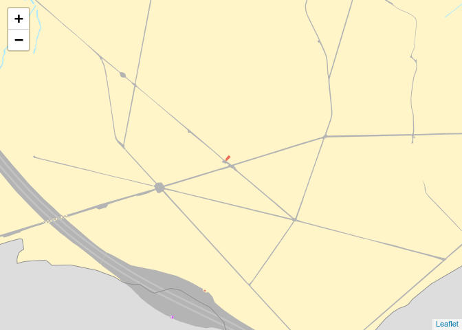
wms_grblinks to the WMS of the GRB-basiskaart, the Flemish cadastral map. It depicts land parcels, buildings, watercourses, roads and railroads. -
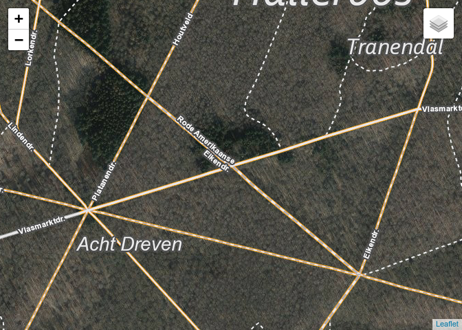
wms_orthocontains a mosaic of recent orthophotos made during the winter. The layerOrthocontains the images, the layerVliegdagcontourdetail on the time when the pictures were taken. -
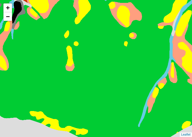
wms_inbois a WMS providing several layers. -
wms_huntingdisplays hunting grounds in Flanders. -
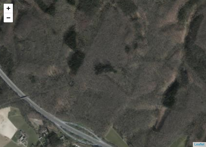
wms_cartoweb_beprovides several cartographic layers from the National Geographic Institute (NGI). -
wms_ortho_beprovides recent orthophotos for the whole Belgian territory, compiled by NGI.
In the WFS tutorial, we present a handy overview of websites with WMS (and WFS) services.
Simple maps
WMS layers can be added to a leaflet map using the addWMSTiles()
function.
It is required to define the map view with setView(), by providing a
map center (as longitude and latitude coordinates) and a zoom level.
leaflet() %>%
  setView(lng = 4.287638, lat = 50.703039, zoom = 15) %>%
  addWMSTiles(
    wms_grb,
    layers = "GRB_BSK",
    options = WMSTileOptions(format = "image/png", transparent = TRUE)
  )
Note: run the code to see this and the following interactive maps.
leaflet() %>%
  setView(lng = 4.287638, lat = 50.703039, zoom = 15) %>%
  addWMSTiles(
    wms_ortho,
    layers = "Ortho",
    options = WMSTileOptions(format = "image/png", transparent = TRUE)
  )
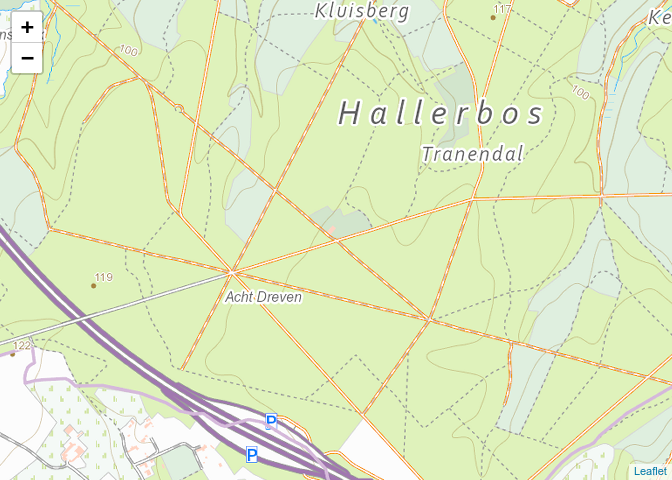
leaflet() %>%
  setView(lng = 4.287638, lat = 50.703039, zoom = 15) %>%
  addWMSTiles(
    wms_inbo,
    layers = "PNVeg",
    options = WMSTileOptions(format = "image/png", transparent = TRUE)
  )
leaflet() %>%
  setView(lng = 4.287638, lat = 50.703039, zoom = 15) %>%
  addWMSTiles(
    wms_cartoweb_be,
    layers = "topo",
    options = WMSTileOptions(format = "image/png")
  )
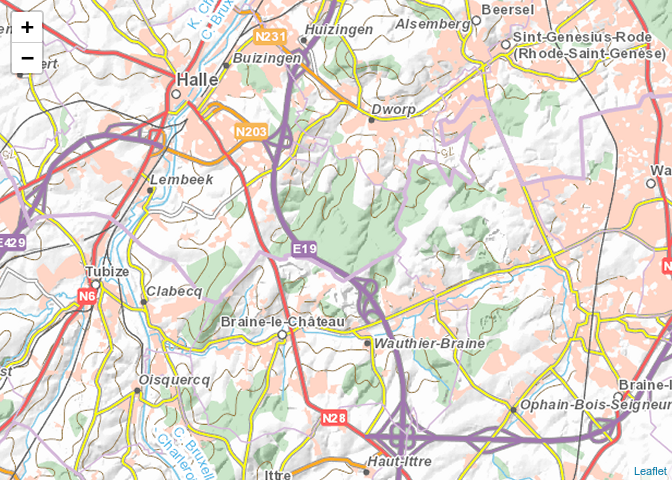
Setting another zoom level of the CartoWeb service triggers the display of another topographic map. Of course you can do that interactively with the above map (not supported on this web site though).
leaflet() %>%
  setView(lng = 4.287638, lat = 50.703039, zoom = 12) %>%
  addWMSTiles(
    wms_cartoweb_be,
    layers = "topo",
    options = WMSTileOptions(format = "image/png")
  )
Combining multiple layers
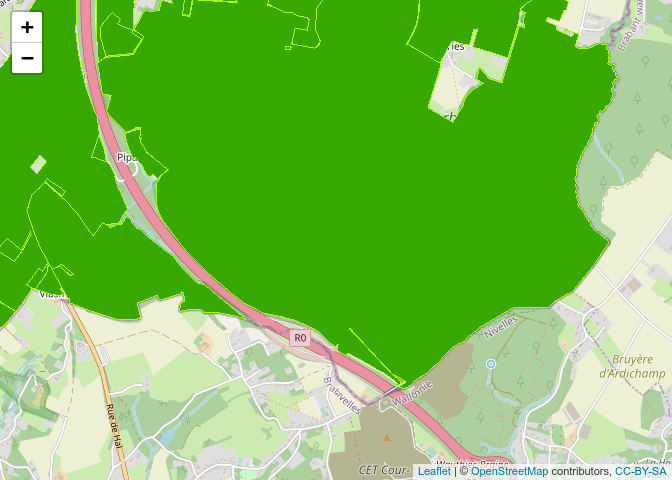
Below, we also add OpenStreetMap in the background.
leaflet() %>%
  setView(lng = 4.287638, lat = 50.703039, zoom = 14) %>%
  addTiles(group = "OSM") %>%
  addWMSTiles(
    wms_hunting,
    layers = "Jachtterr",
    options = WMSTileOptions(format = "image/png", transparent = TRUE)
  )
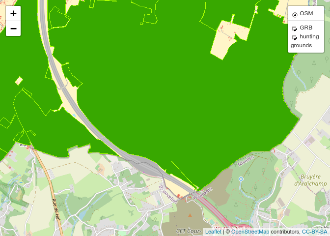
By adding addWMSTiles() multiple times, several WMSs can be displayed
on top of each other.
leaflet() %>%
  setView(lng = 4.287638, lat = 50.703039, zoom = 14) %>%
  addTiles(group = "OSM") %>%
  addWMSTiles(
    wms_grb,
    layers = "GRB_BSK",
    options = WMSTileOptions(format = "image/png", transparent = TRUE),
    group = "GRB"
  ) %>%
  addWMSTiles(
    wms_hunting,
    layers = "Jachtterr",
    options = WMSTileOptions(format = "image/png", transparent = TRUE),
    group = "hunting<br>grounds"
  ) %>%
  addLayersControl(
    baseGroups = "OSM",
    overlayGroups = c("GRB", "hunting<br>grounds"),
    options = layersControlOptions(collapsed = FALSE)
  )
The overlay layer of the NGI CartoWeb service is aimed at higher zoom
levels and is useful to put on top of a map. Here we take the NGI
orthophoto service as a background map. We must set the overlay layer
transparent in order to see the layers below – the default option being
transparent = FALSE.
leaflet() %>%
  setView(lng = 4.287638, lat = 50.703039, zoom = 16) %>%
  addWMSTiles(
    wms_ortho_be,
    layers = "orthoimage_coverage",
    group = "Orthophoto BE") %>%
  addWMSTiles(
    wms_cartoweb_be,
    layers = "overlay",
    options = WMSTileOptions(format = "image/png", transparent = TRUE),
    group = "Topo BE"
  ) %>%
  addLayersControl(
    baseGroups = "Orthophoto BE",
    overlayGroups = "Topo BE"
  )