Available themes in INBOtheme

Thierry Onkelinx

Introduction

This vignette focuses on the available ggplot2 themes in INBOtheme. They mainly control the looks of the axes, background, legend, … Some themes also impact the schemes when using a colour or fill along a variable. We illustrate that in vignette("colour", package = "INBOtheme").

Important

The ggplot2 package must be loaded prior to INBOtheme. Loading INBOtheme sets inbo_theme() as default theme and inbo_steun_blauw as default colour for the geoms. Note how we use theme_set() and switch_colour(). This applies the theme and colour to all subsequent plots without the need to change the ggplot2 code.

Using the default theme from INBOtheme

Add the following code after loading the ggplot2 or tidyverse package and before creating the ggplot2 plots.

library(INBOtheme)

In case you need to change the default font size or background add the code below after loading the package.

theme_set(theme_inbo(base_size = 12, transparent = FALSE))

Using a non-default theme from INBOtheme

Add the following code after loading the ggplot2 or tidyverse package and before creating the ggplot2 plots.

library(INBOtheme)
theme_set(theme_vlaanderen2015(base_size = 12, transparent = FALSE))
switch_colour(vl_darkyellow)

library(INBOtheme)
theme_set(theme_elsevier(base_size = 12, transparent = FALSE))
switch_colour("black")

Prepare the code and data

library(ggplot2)
library(INBOtheme)

# Prepare the data for the figures
d <- data.frame(
  x = "Sphinx of black quartz, judge my vow",
  y = "Sphinx of\nblack quartz,\njudge my vow"
)
data("esoph")
cancer <- esoph
cancer$Age <- cancer$agegp
cancer$Alcohol <- cancer$alcgp
cancer$Tabacco <- cancer$tobgp
cancer$Proportion <- cancer$ncases / (cancer$ncases + cancer$ncontrols)

Default: theme_inbo()

theme_inbo() with default background

theme_set(theme_inbo(base_size = 12))
switch_colour(inbo_steun_blauw)

ggplot(d, aes(x = x, y = x, label = y)) +
  geom_text(size = 8) +
  labs(x = d$x, y = d$x, title = d$x, colour = d$y) +
  theme(axis.text.y = element_text(angle = 90, hjust = 0.5))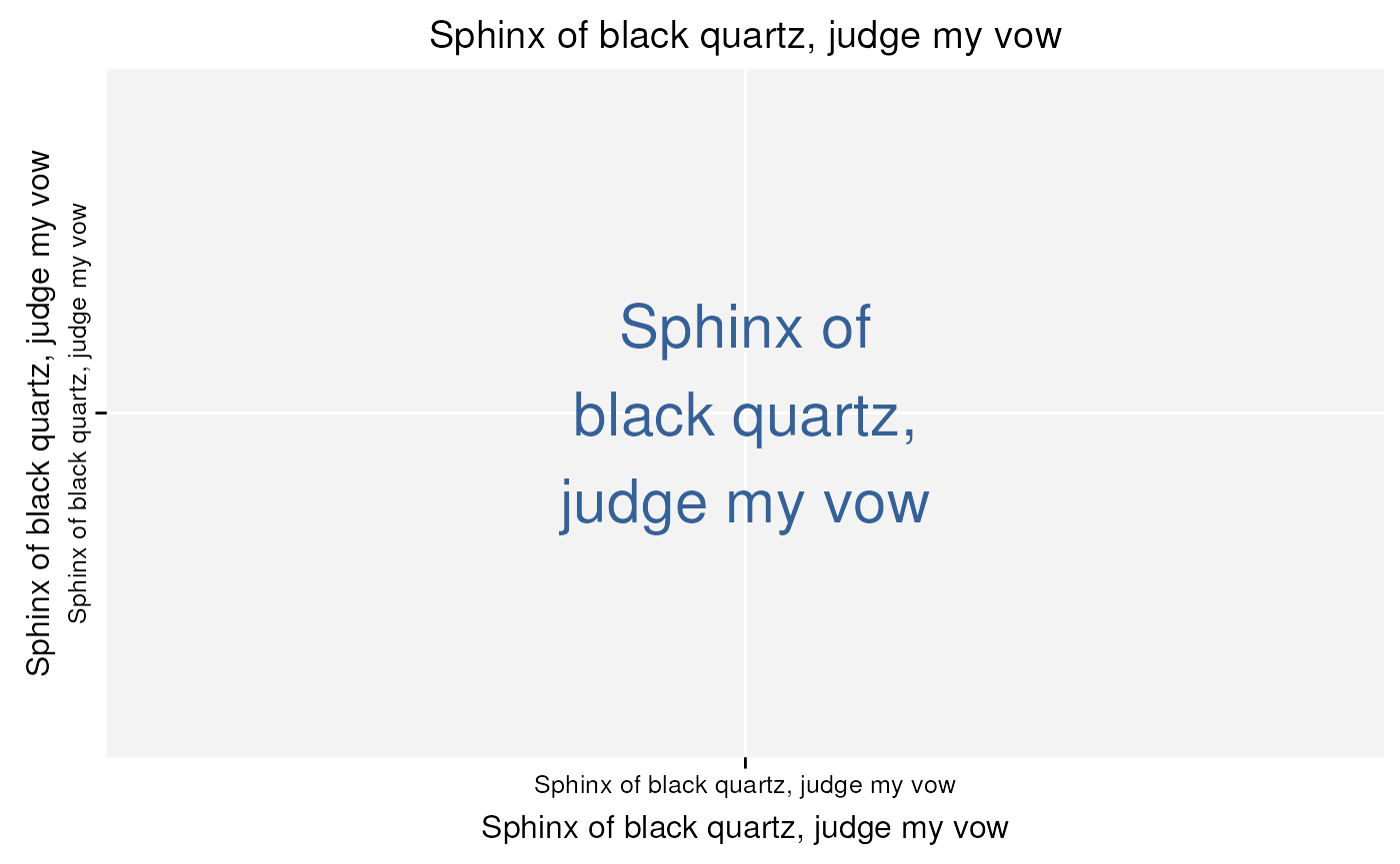

Testing fonts.

ggplot(cancer, aes(x = Age, y = Proportion)) +
  geom_boxplot() +
  ggtitle("cancer dataset")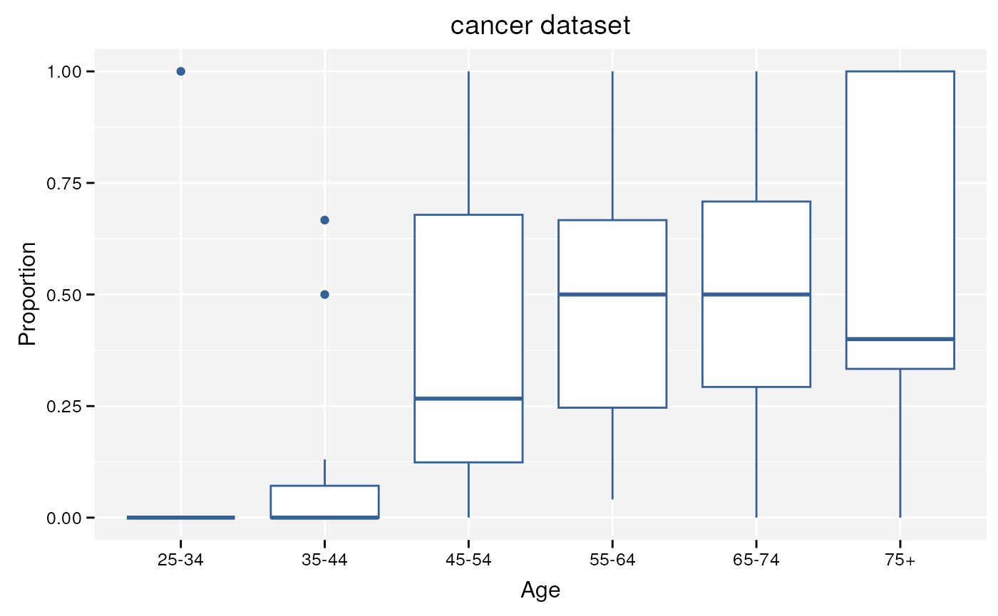

geom_boxplot()

ggplot(cancer, aes(x = Proportion)) +
  geom_histogram(binwidth = 0.05) +
  facet_wrap(~Age, scales = "free") +
  ggtitle("cancer dataset")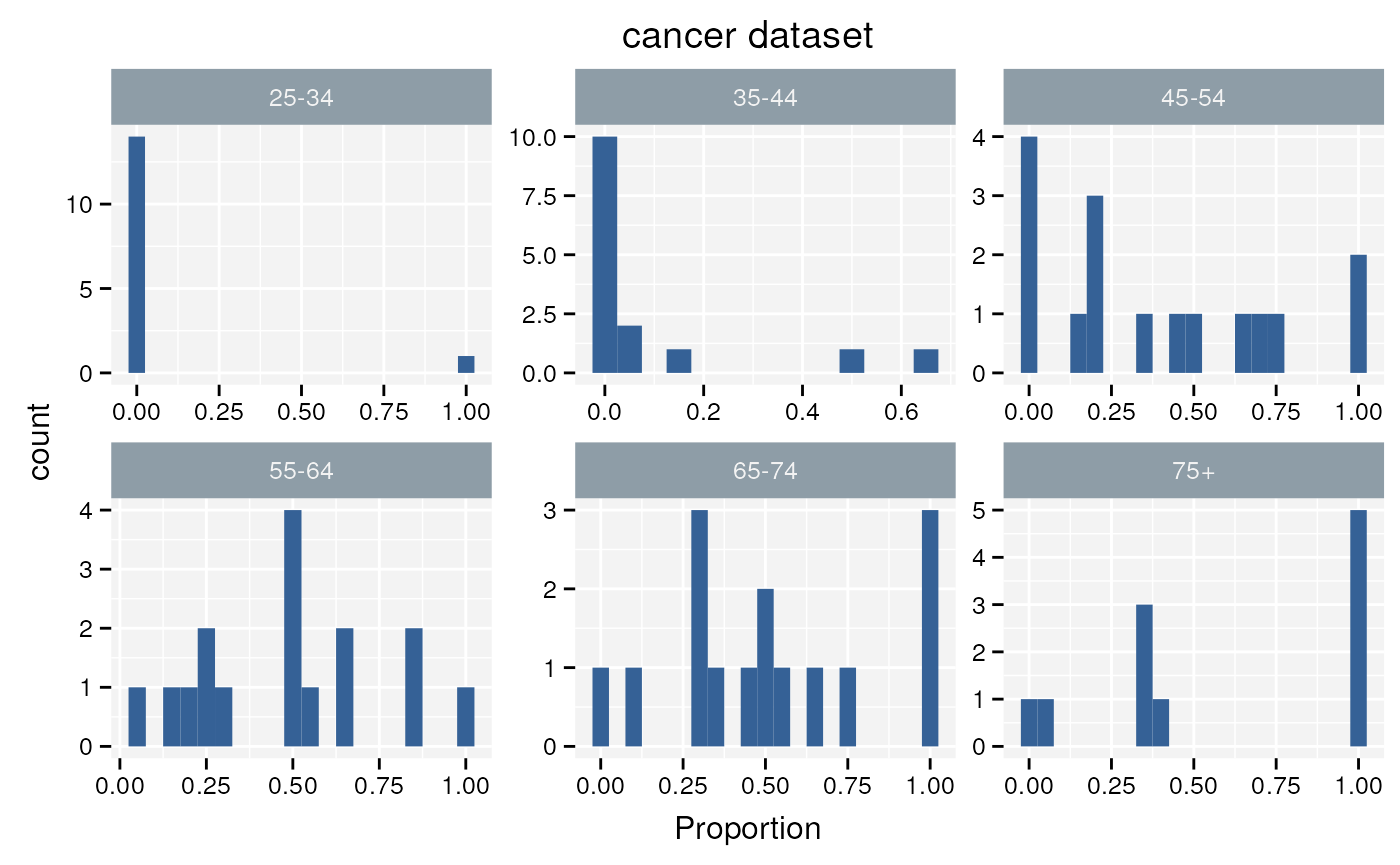

Histogram split into subplots with facet_wrap().

ggplot(cancer, aes(x = Proportion)) +
  geom_histogram(binwidth = 0.05) +
  facet_grid(alcgp ~ tobgp, scales = "free") +
  ggtitle("cancer dataset")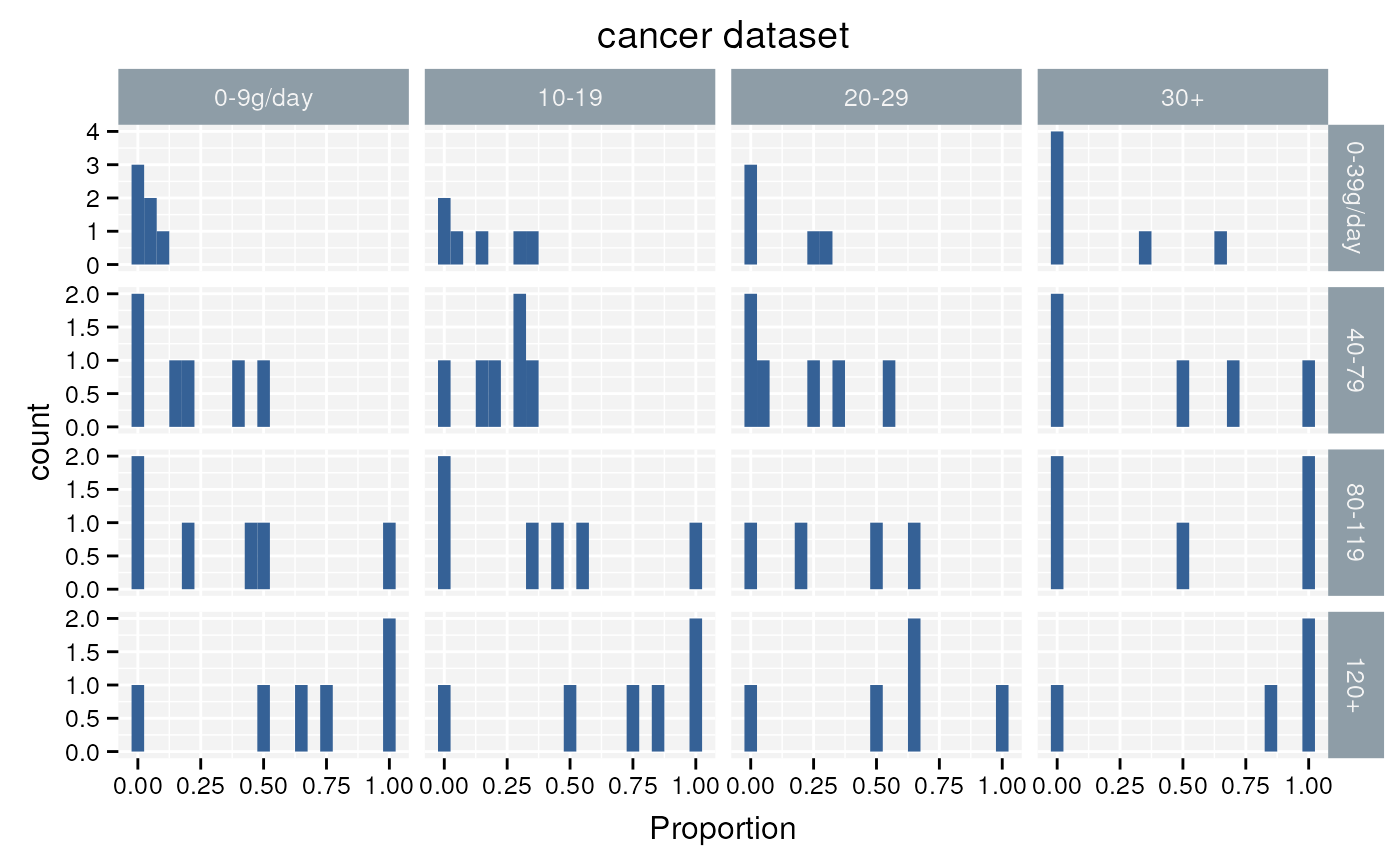

Histogram split into subplots with facet_grid().

theme_inbo() with transparent background

theme_set(theme_inbo(base_size = 12, transparent = TRUE))
switch_colour(inbo_steun_blauw)

ggplot(d, aes(x = x, y = x, label = y)) +
  geom_text(size = 8) +
  labs(x = d$x, y = d$x, title = d$x, colour = d$y) +
  theme(axis.text.y = element_text(angle = 90, hjust = 0.5))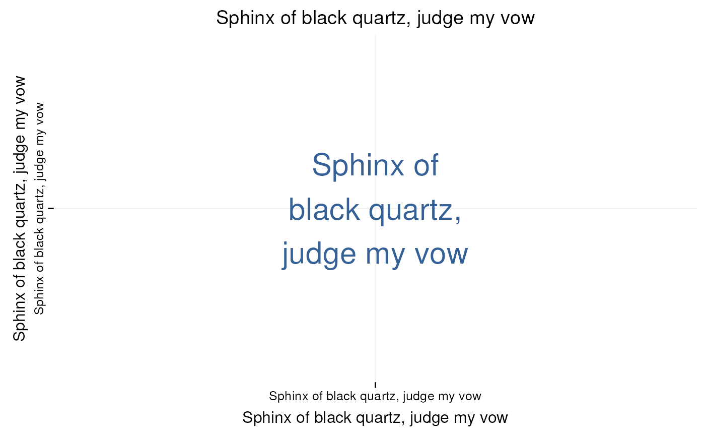

Testing fonts.

ggplot(cancer, aes(x = Age, y = Proportion)) +
  geom_boxplot() +
  ggtitle("cancer dataset")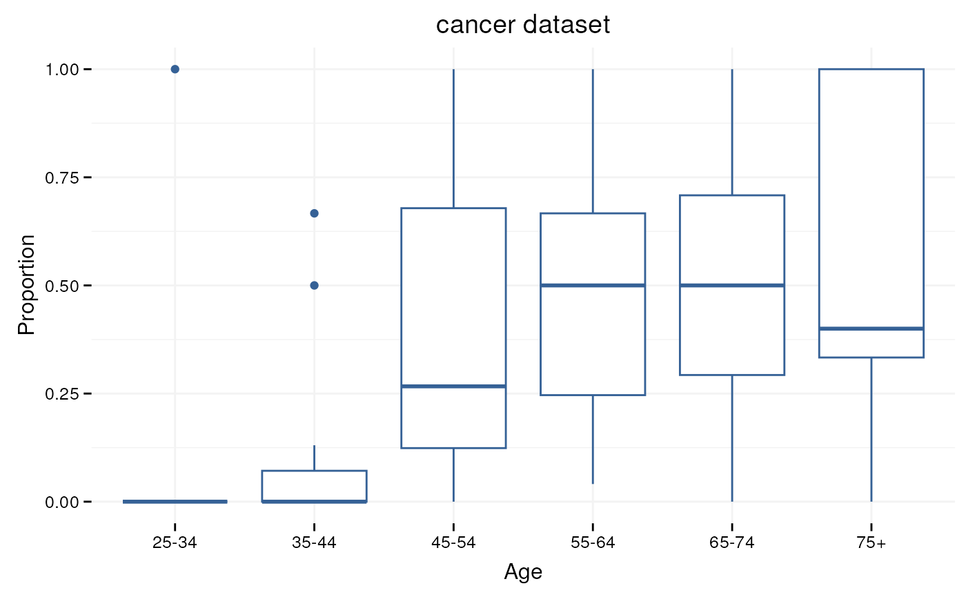

geom_boxplot()

ggplot(cancer, aes(x = Proportion)) +
  geom_histogram(binwidth = 0.05) +
  facet_wrap(~Age, scales = "free") +
  ggtitle("cancer dataset")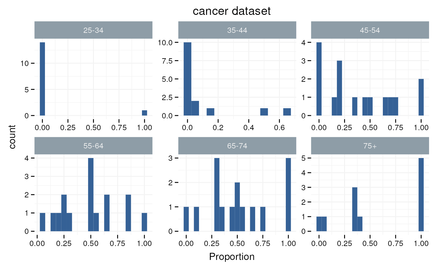

Histogram split into subplots with facet_wrap().

ggplot(cancer, aes(x = Proportion)) +
  geom_histogram(binwidth = 0.05) +
  facet_grid(alcgp ~ tobgp, scales = "free") +
  ggtitle("cancer dataset")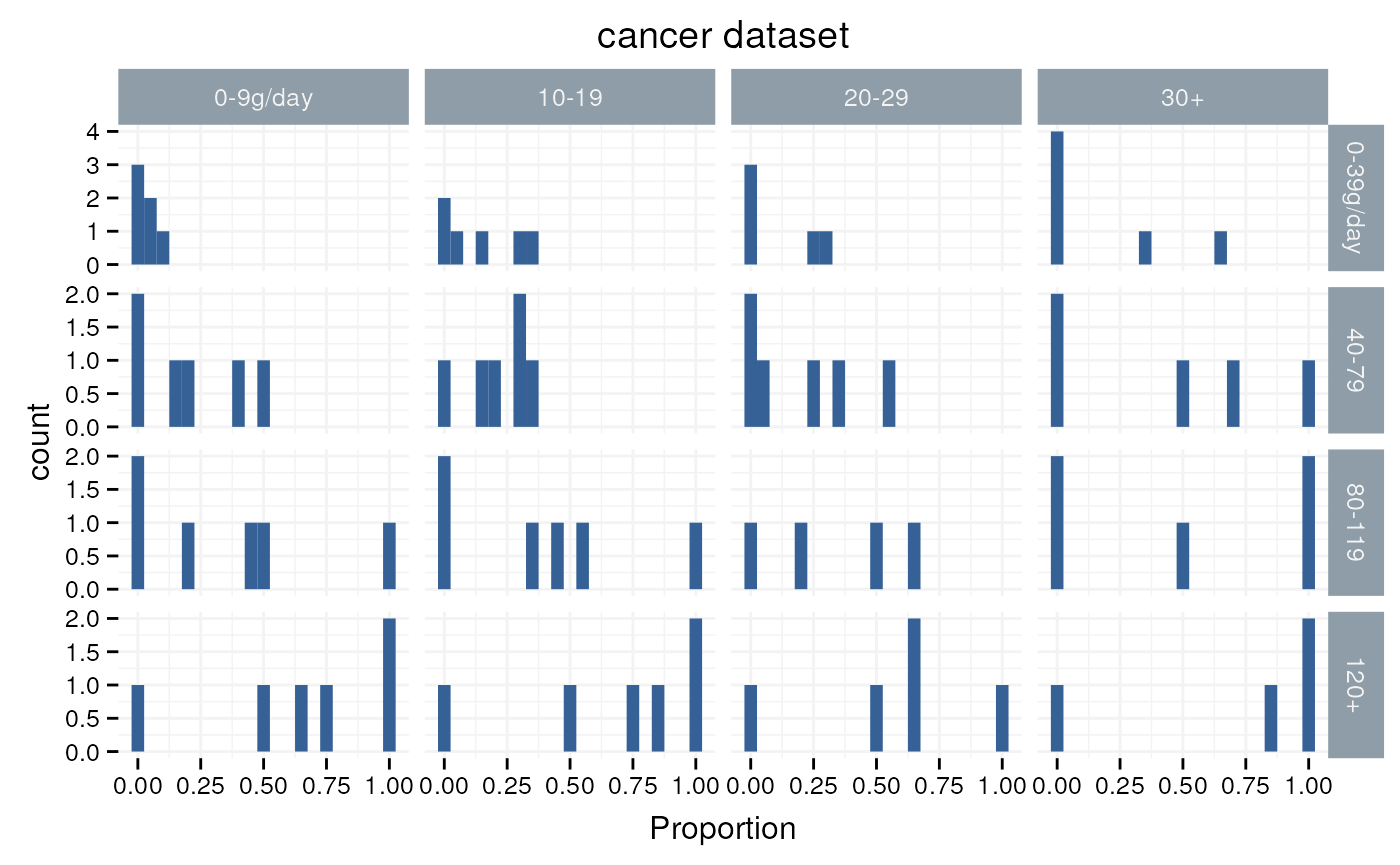

Histogram split into subplots with facet_grid().

theme_vlaanderen2015()

theme_vlaanderen2015() with default background

theme_set(theme_vlaanderen2015(base_size = 12))
switch_colour(vl_darkyellow)

ggplot(d, aes(x = x, y = x, label = y)) +
  geom_text(size = 8) +
  labs(x = d$x, y = d$x, title = d$x, colour = d$y) +
  theme(axis.text.y = element_text(angle = 90, hjust = 0.5))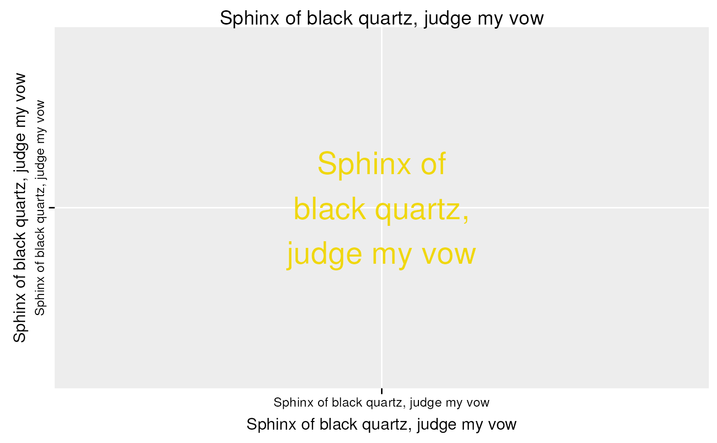

Testing fonts.

ggplot(cancer, aes(x = Age, y = Proportion)) +
  geom_boxplot() +
  ggtitle("cancer dataset")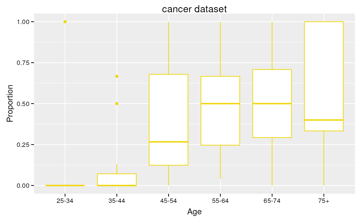

geom_boxplot()

ggplot(cancer, aes(x = Proportion)) +
  geom_histogram(binwidth = 0.05) +
  facet_wrap(~Age, scales = "free") +
  ggtitle("cancer dataset")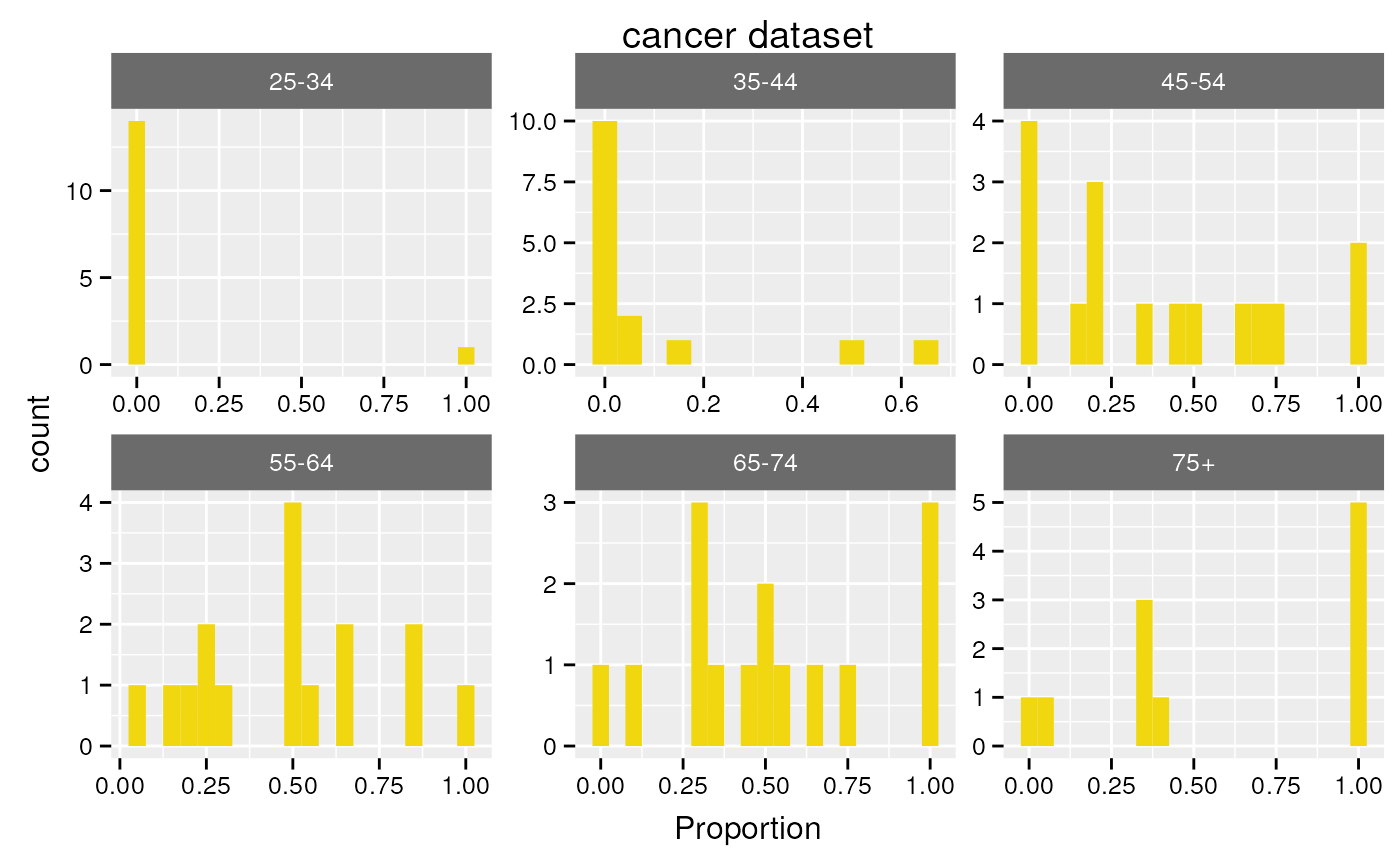

Histogram split into subplots with facet_wrap().

ggplot(cancer, aes(x = Proportion)) +
  geom_histogram(binwidth = 0.05) +
  facet_grid(alcgp ~ tobgp, scales = "free") +
  ggtitle("cancer dataset")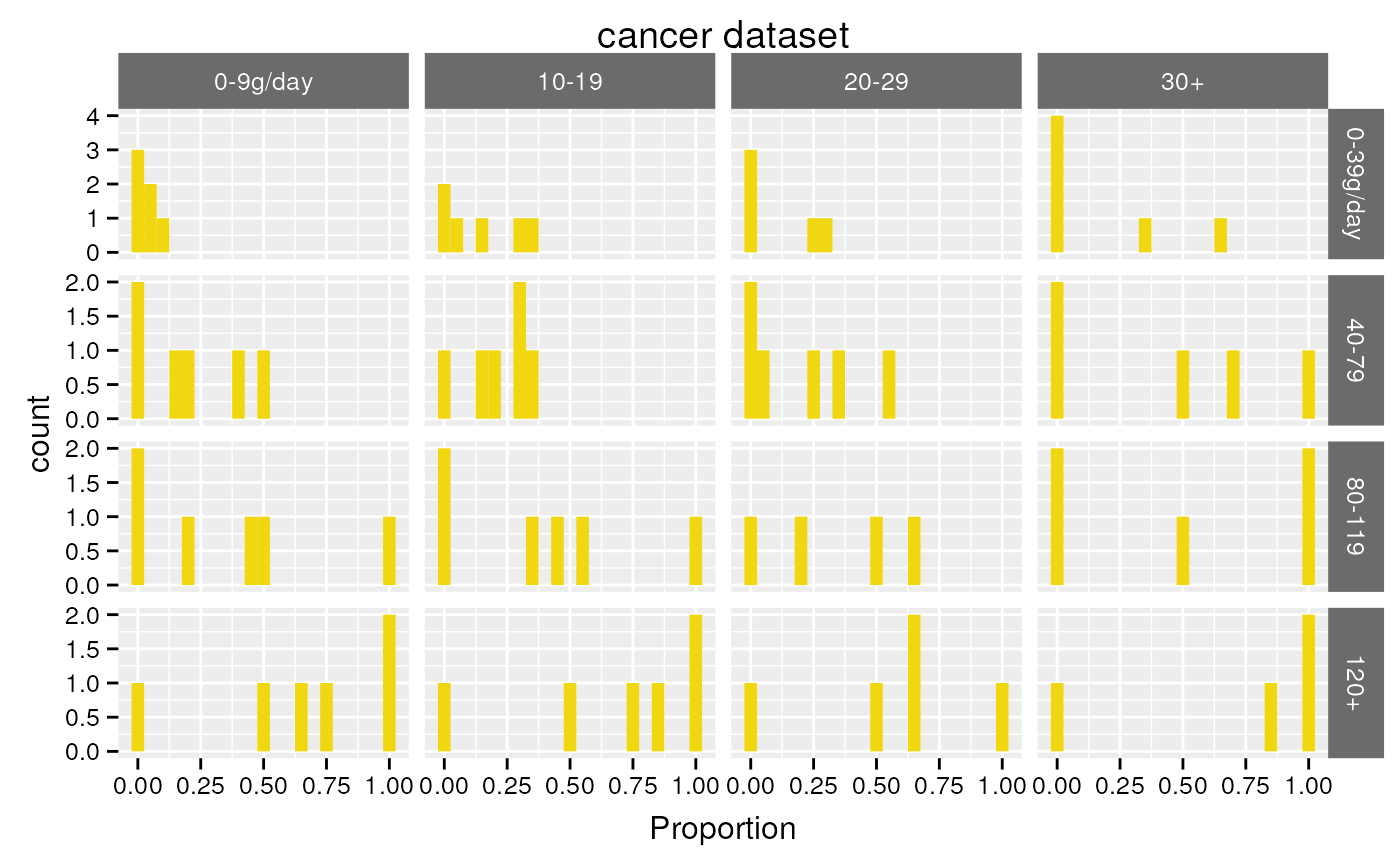

Histogram split into subplots with facet_grid().

theme_vlaanderen2015() with transparent background

theme_set(theme_vlaanderen2015(base_size = 12, transparent = TRUE))
switch_colour(vl_darkyellow)

ggplot(d, aes(x = x, y = x, label = y)) +
  geom_text(size = 8) +
  labs(x = d$x, y = d$x, title = d$x, colour = d$y) +
  theme(axis.text.y = element_text(angle = 90, hjust = 0.5))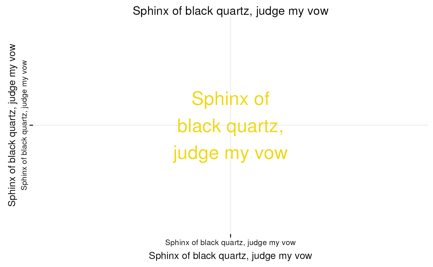

Testing fonts.

ggplot(cancer, aes(x = Age, y = Proportion)) +
  geom_boxplot() +
  ggtitle("cancer dataset")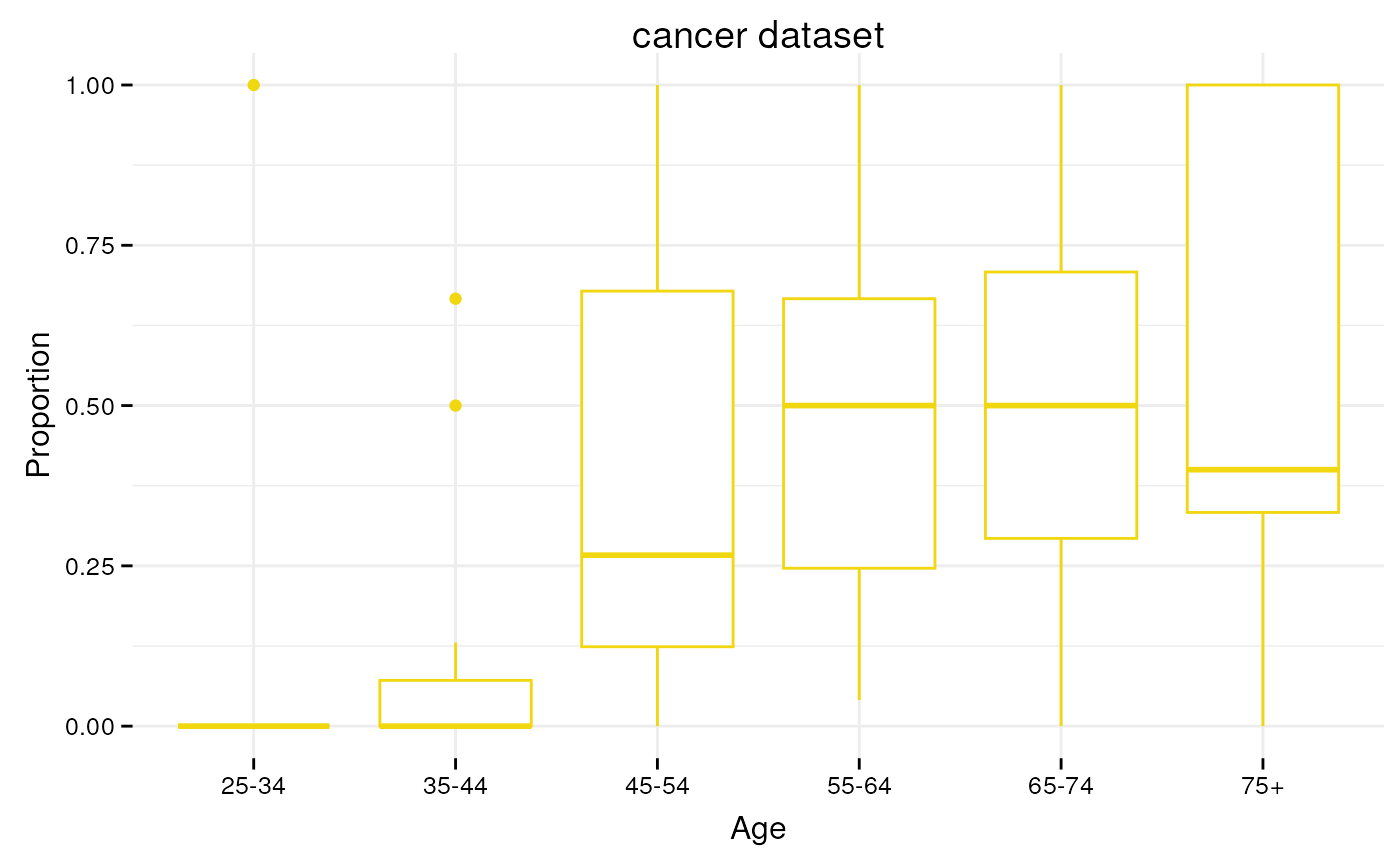

geom_boxplot()

ggplot(cancer, aes(x = Proportion)) +
  geom_histogram(binwidth = 0.05) +
  facet_wrap(~Age, scales = "free") +
  ggtitle("cancer dataset")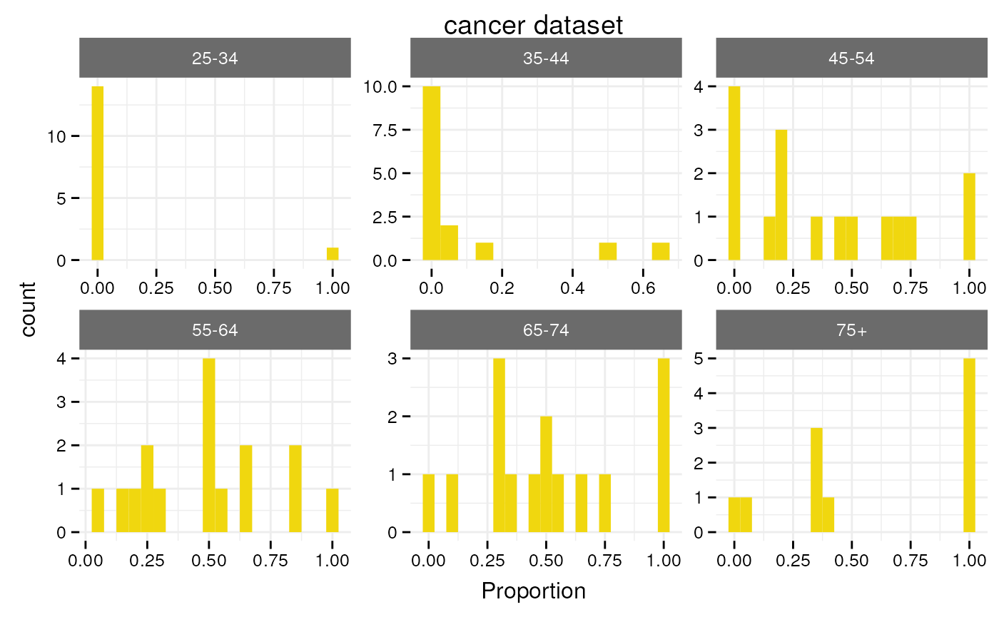

Histogram split into subplots with facet_wrap().

ggplot(cancer, aes(x = Proportion)) +
  geom_histogram(binwidth = 0.05) +
  facet_grid(alcgp ~ tobgp, scales = "free") +
  ggtitle("cancer dataset")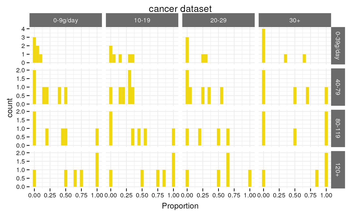

Histogram split into subplots with facet_grid().

theme_elsevier()

Note that theme_elsevier() uses a base font size of 7. Use that default when preparing plots for a paper.

theme_set(theme_elsevier(base_size = 12))
switch_colour("black")

ggplot(d, aes(x = x, y = x, label = y)) +
  geom_text(size = 8) +
  labs(x = d$x, y = d$x, title = d$x, colour = d$y) +
  theme(axis.text.y = element_text(angle = 90, hjust = 0.5))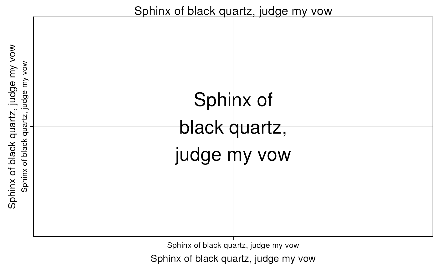

Testing fonts.

ggplot(cancer, aes(x = Age, y = Proportion)) +
  geom_boxplot() +
  ggtitle("cancer dataset")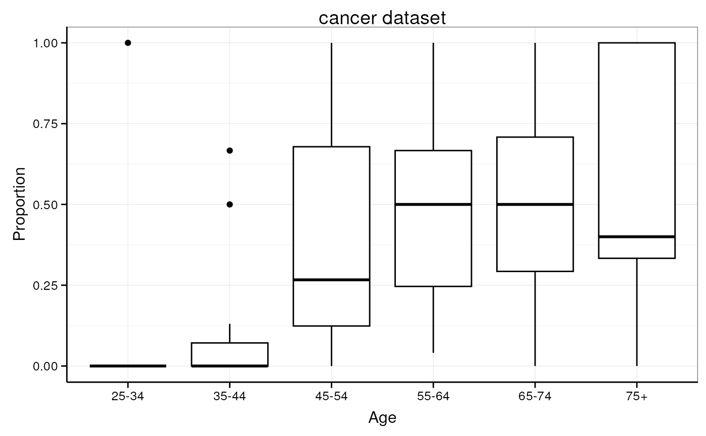

geom_boxplot()

ggplot(cancer, aes(x = Proportion)) +
  geom_histogram(binwidth = 0.05) +
  facet_wrap(~Age, scales = "free") +
  ggtitle("cancer dataset")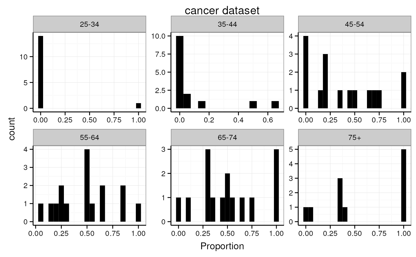

Histogram split into subplots with facet_wrap().

ggplot(cancer, aes(x = Proportion)) +
  geom_histogram(binwidth = 0.05) +
  facet_grid(alcgp ~ tobgp, scales = "free") +
  ggtitle("cancer dataset")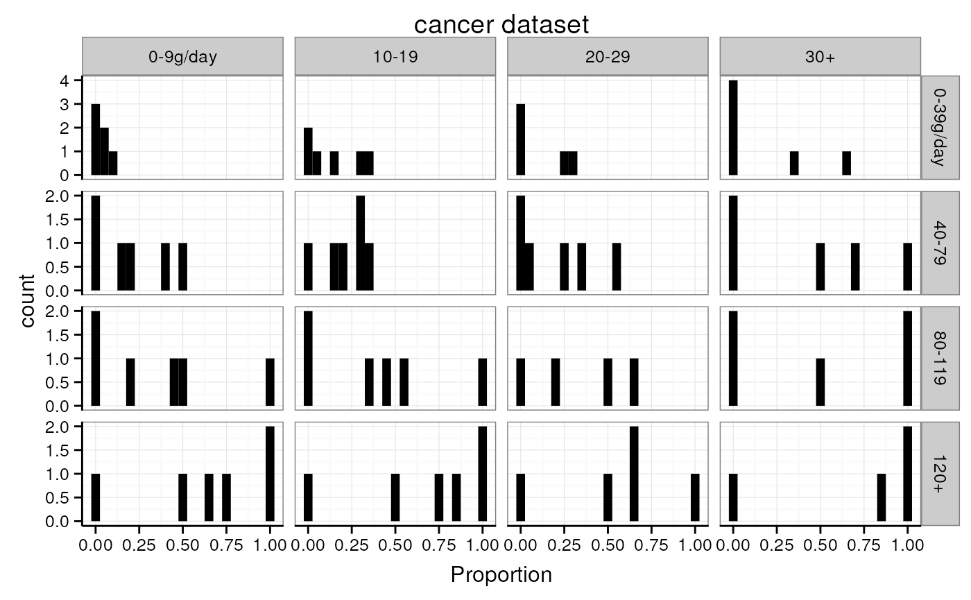

Histogram split into subplots with facet_grid().