Default colours along a variable in INBOtheme
Thierry Onkelinx
Source:vignettes/colour.Rmd
colour.RmdIntroduction
Some themes impact the scales when using a colour or fill along a
variable. This vignette focusses on the different styles of colour
scales. The fill scales uses the same gradients. To keep the vignette
small, we only give examples with different colours. We illustrate the
other effects of the themes in
vignette("colour", package = "INBOtheme"), again to keep
the size of the vignettes to a minimum. Note that you need to use the
appropriate scale provided by INBOtheme in case of a
gradient along a continuous variable.
Default: theme_inbo()
Continuous variable
ggplot(diamonds, aes(x = carat, y = depth, colour = price)) +
  geom_point() +
  scale_colour_gradient()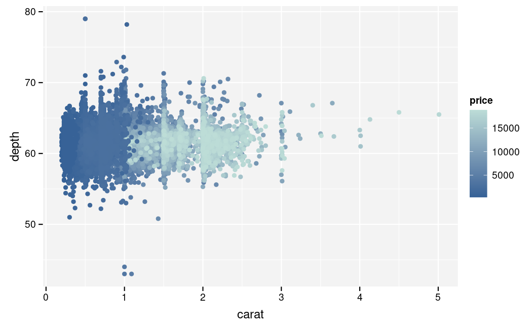
Coloured along a continuous variable.
ggplot(diamonds, aes(x = carat, y = depth, colour = price)) +
  geom_point() +
  scale_colour_gradient2(midpoint = 1e4)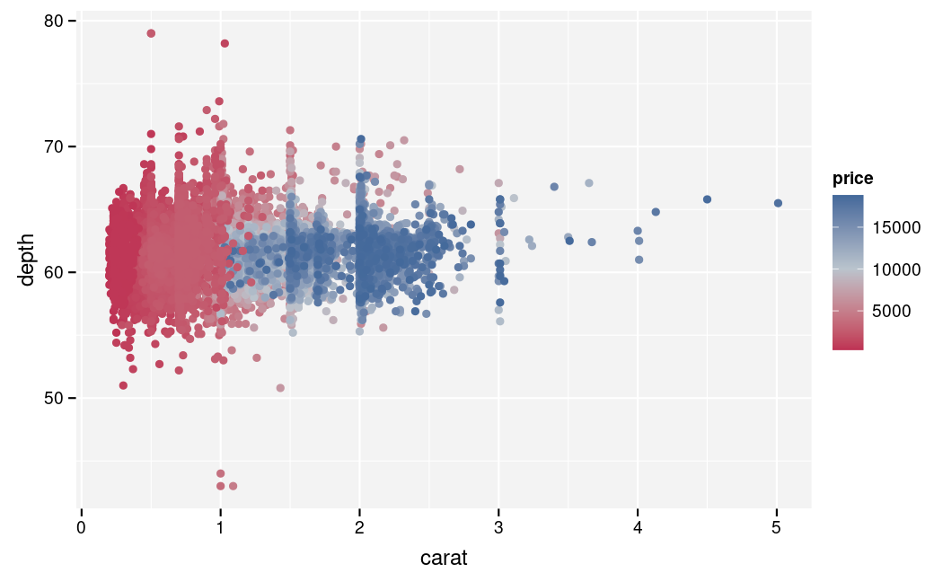
Coloured along a continuous variable using a gradient with midpoint.
Ordinal variable
ggplot(diamonds, aes(x = carat, y = depth, colour = cut)) +
  geom_point()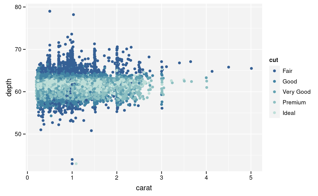
Coloured along an ordinal variable.
Categorical variable
Here we illustrate figures with a different number of categories. We choose for scatter plots with random x, y and category. This is the most difficult situation to distinguish the colours. Be careful when you use more than 5 colours.
data.frame(
  x = runif(1e3), y = runif(1e3),
  category = sample(LETTERS[1:2], 1e3, replace = TRUE)
) |>
  ggplot(aes(x = x, y = y, colour = category)) +
  geom_jitter()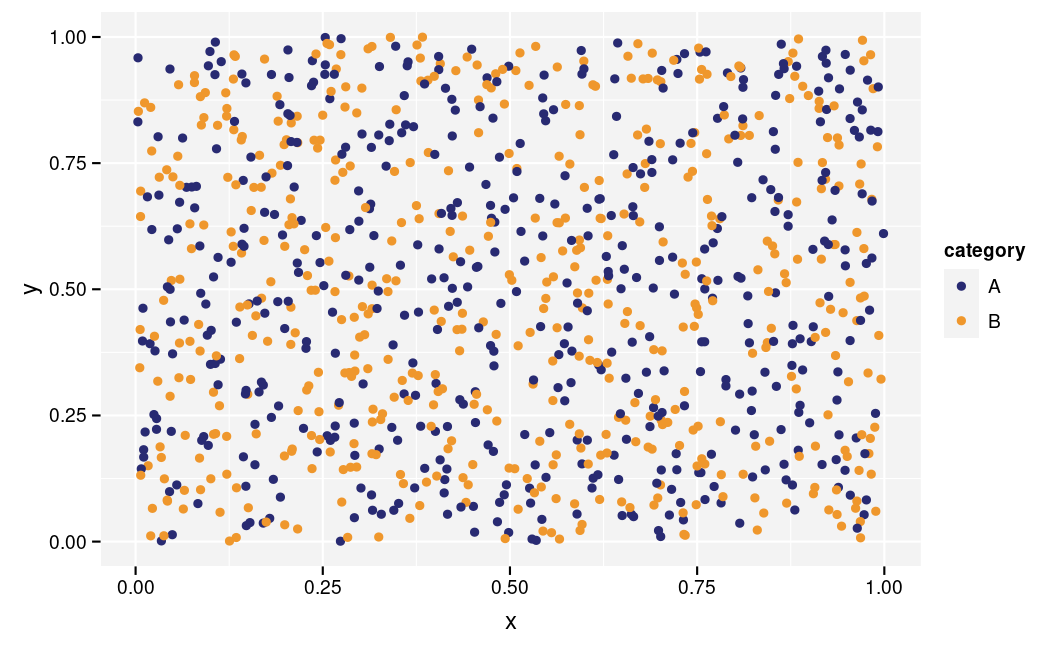
Coloured by a two level categorical variable.
data.frame(
  x = runif(1e3), y = runif(1e3),
  category = sample(LETTERS[1:3], 1e3, replace = TRUE)
) |>
  ggplot(aes(x = x, y = y, colour = category)) +
  geom_jitter()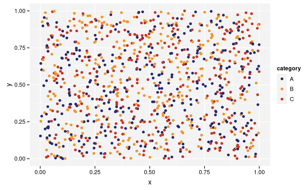
Coloured by a three level categorical variable.
data.frame(
  x = runif(1e3), y = runif(1e3),
  category = sample(LETTERS[1:4], 1e3, replace = TRUE)
) |>
  ggplot(aes(x = x, y = y, colour = category)) +
  geom_jitter()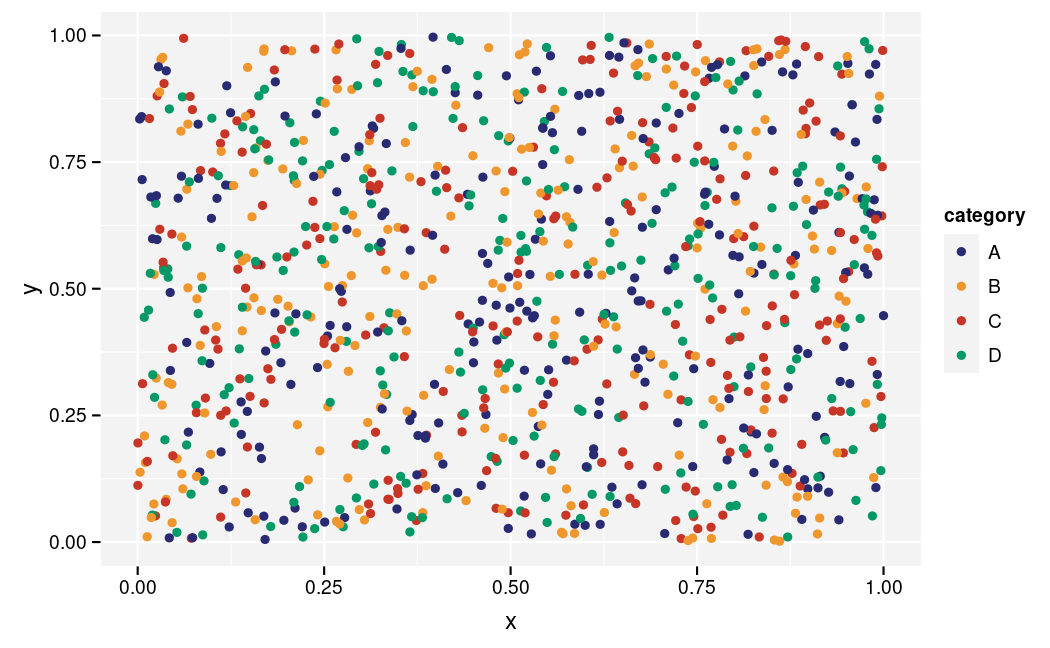
Coloured by a four level categorical variable.
data.frame(
  x = runif(1e3), y = runif(1e3),
  category = sample(LETTERS[1:5], 1e3, replace = TRUE)
) |>
  ggplot(aes(x = x, y = y, colour = category)) +
  geom_jitter()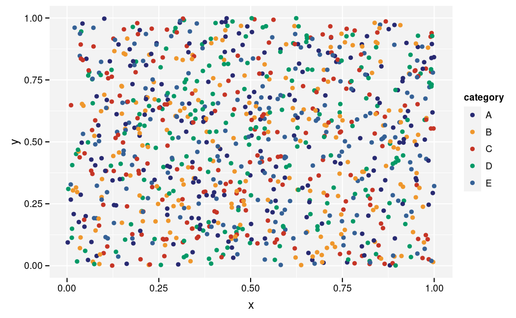
Coloured by a five level categorical variable.
data.frame(
  x = runif(1e3), y = runif(1e3),
  category = sample(LETTERS[1:6], 1e3, replace = TRUE)
) |>
  ggplot(aes(x = x, y = y, colour = category)) +
  geom_jitter()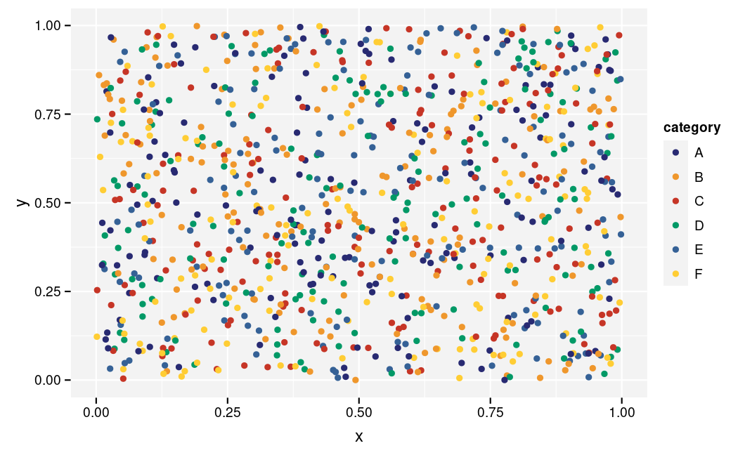
Coloured by a six level categorical variable.
data.frame(
  x = runif(1e3), y = runif(1e3),
  category = sample(LETTERS[1:7], 1e3, replace = TRUE)
) |>
  ggplot(aes(x = x, y = y, colour = category)) +
  geom_jitter()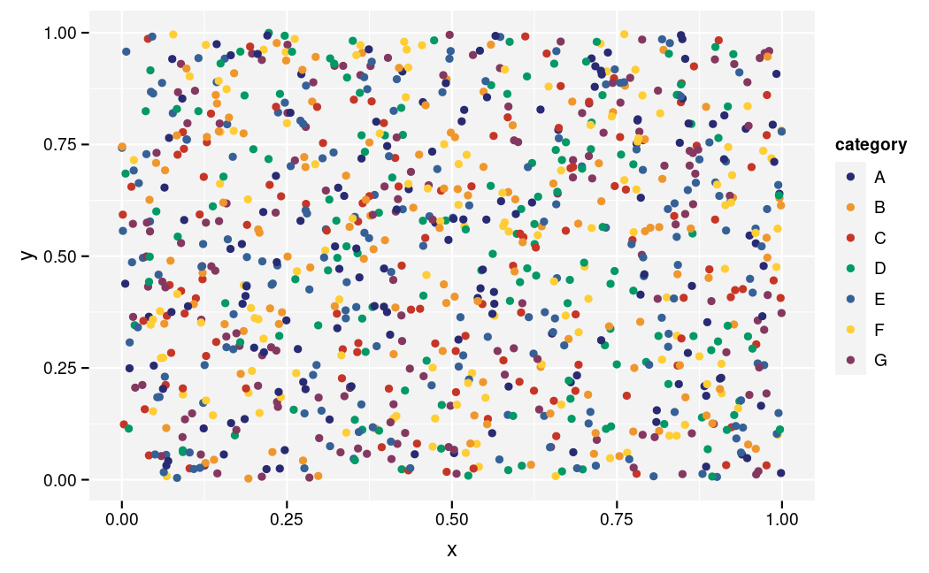
Coloured by a seven level categorical variable.
data.frame(
  x = runif(1e3), y = runif(1e3),
  category = sample(LETTERS[1:8], 1e3, replace = TRUE)
) |>
  ggplot(aes(x = x, y = y, colour = category)) +
  geom_jitter()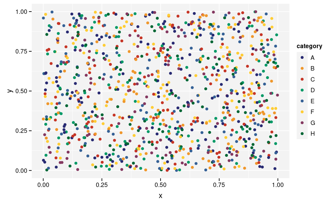
Coloured by an eight level categorical variable.
theme_vlaanderen2015()
Continuous variable
ggplot(diamonds, aes(x = carat, y = depth, colour = price)) +
  geom_point() +
  scale_colour_gradient()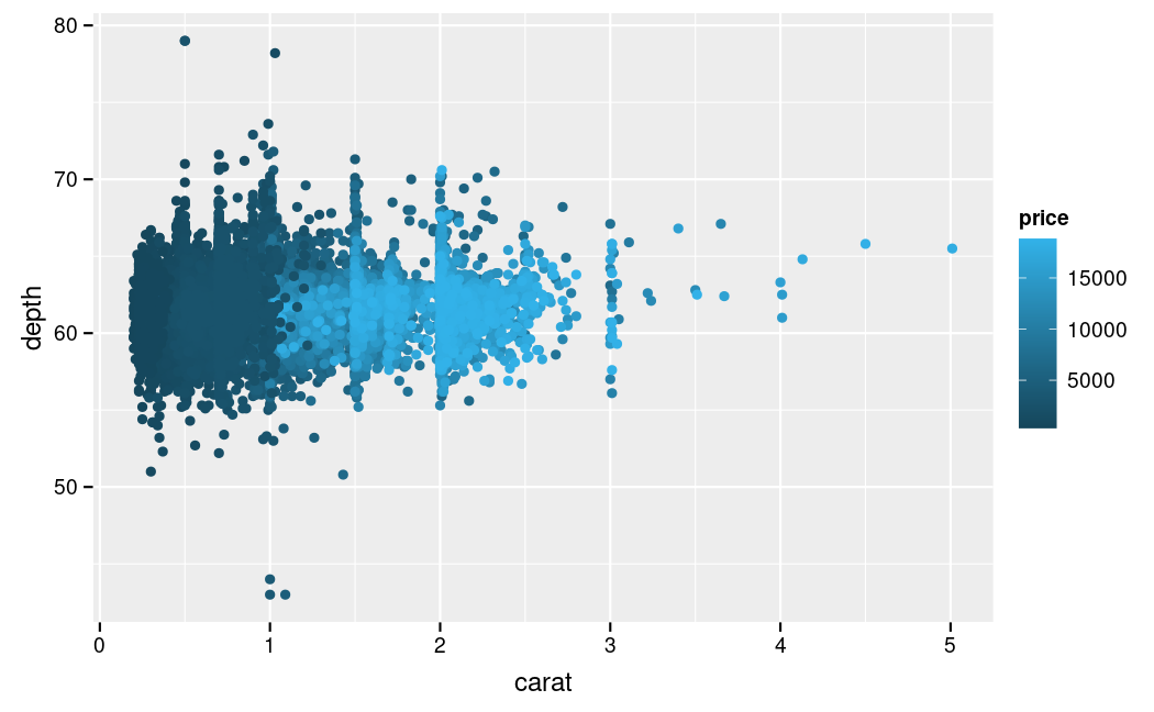
Coloured along a continuous variable.
ggplot(diamonds, aes(x = carat, y = depth, colour = price)) +
  geom_point() +
  scale_colour_gradient2(midpoint = 1e4)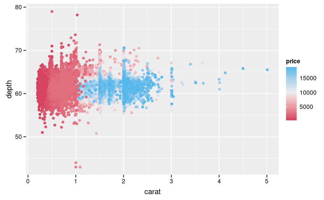
Coloured along a continuous variable using a gradient with midpoint.
Ordinal variable
ggplot(diamonds, aes(x = carat, y = depth, colour = cut)) +
  geom_point()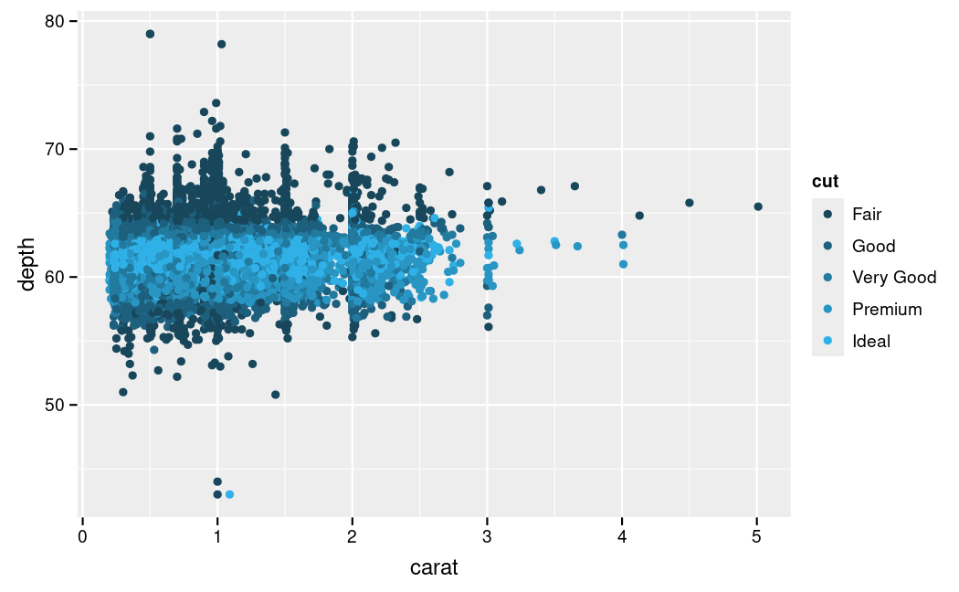
Coloured along an ordinal variable.
Categorical variable
Here we illustrate figures with a different number of categories. We choose for scatter plots with random x, y and category. This is the most difficult situation to distinguish the colours. Be careful when you use more than 5 colours.
data.frame(
  x = runif(1e3), y = runif(1e3),
  category = sample(LETTERS[1:2], 1e3, replace = TRUE)
) |>
  ggplot(aes(x = x, y = y, colour = category)) +
  geom_jitter()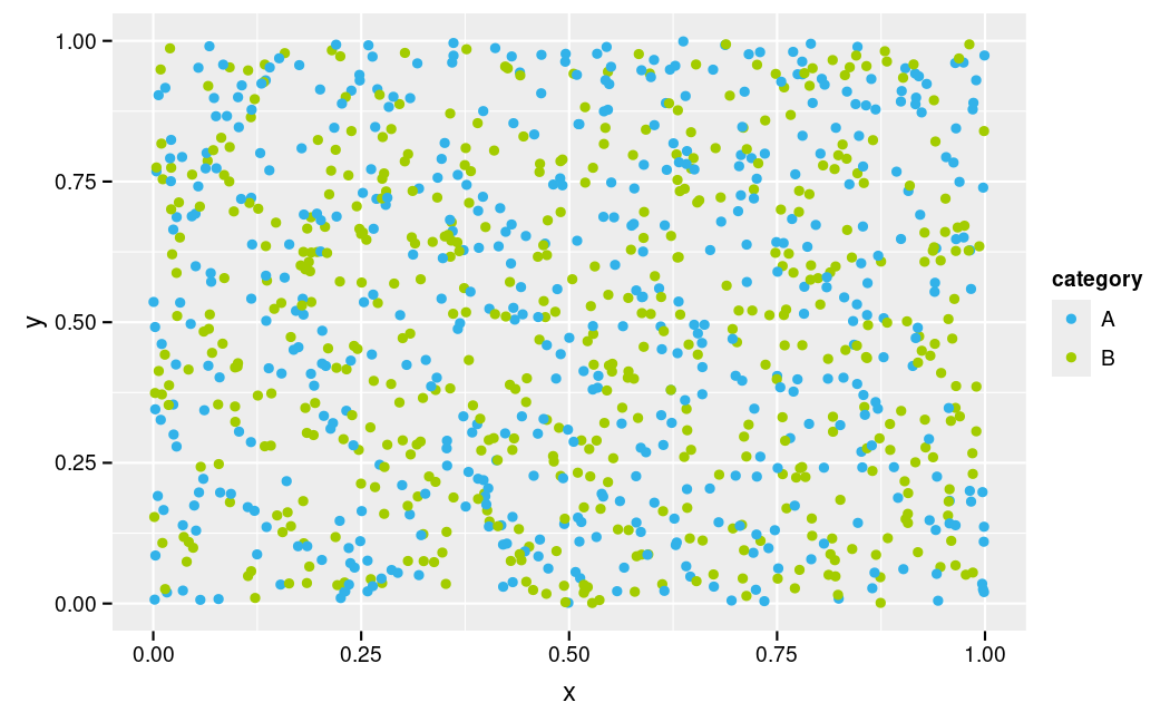
Coloured by a two level categorical variable.
data.frame(
  x = runif(1e3), y = runif(1e3),
  category = sample(LETTERS[1:3], 1e3, replace = TRUE)
) |>
  ggplot(aes(x = x, y = y, colour = category)) +
  geom_jitter()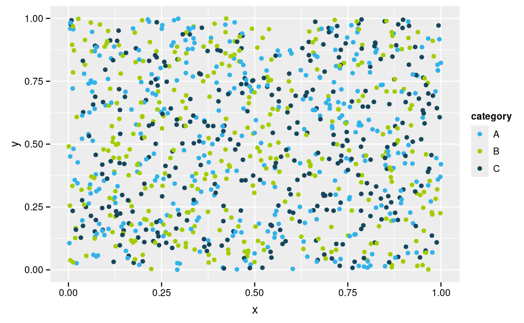
Coloured by a three level categorical variable.
data.frame(
  x = runif(1e3), y = runif(1e3),
  category = sample(LETTERS[1:4], 1e3, replace = TRUE)
) |>
  ggplot(aes(x = x, y = y, colour = category)) +
  geom_jitter()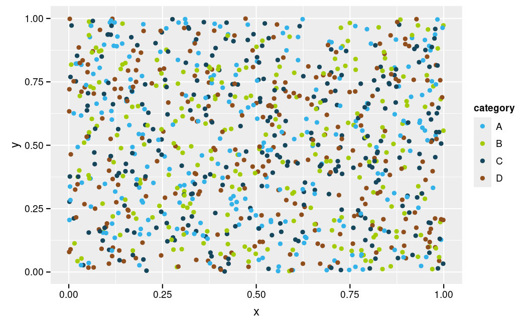
Coloured by a four level categorical variable.
data.frame(
  x = runif(1e3), y = runif(1e3),
  category = sample(LETTERS[1:5], 1e3, replace = TRUE)
) |>
  ggplot(aes(x = x, y = y, colour = category)) +
  geom_jitter()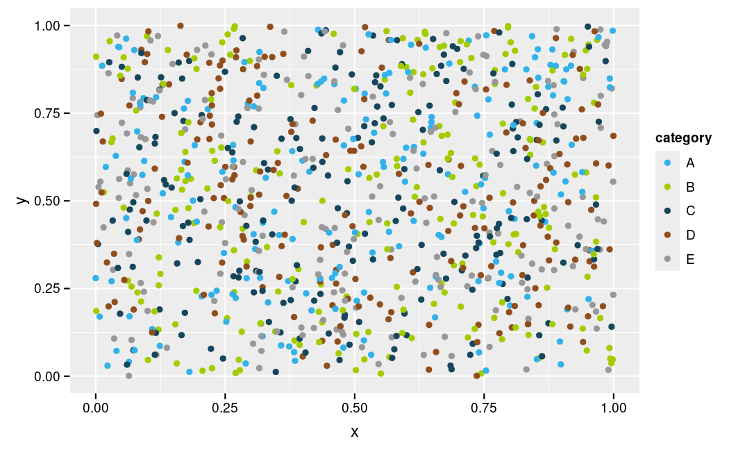
Coloured by a five level categorical variable.
data.frame(
  x = runif(1e3), y = runif(1e3),
  category = sample(LETTERS[1:6], 1e3, replace = TRUE)
) |>
  ggplot(aes(x = x, y = y, colour = category)) +
  geom_jitter()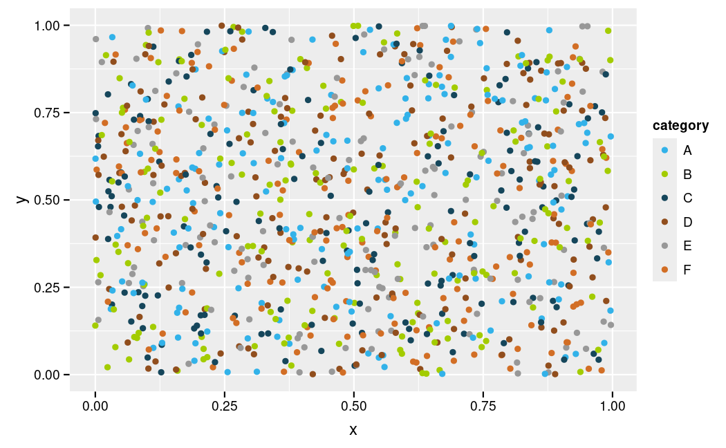
Coloured by a six level categorical variable.
data.frame(
  x = runif(1e3), y = runif(1e3),
  category = sample(LETTERS[1:7], 1e3, replace = TRUE)
) |>
  ggplot(aes(x = x, y = y, colour = category)) +
  geom_jitter()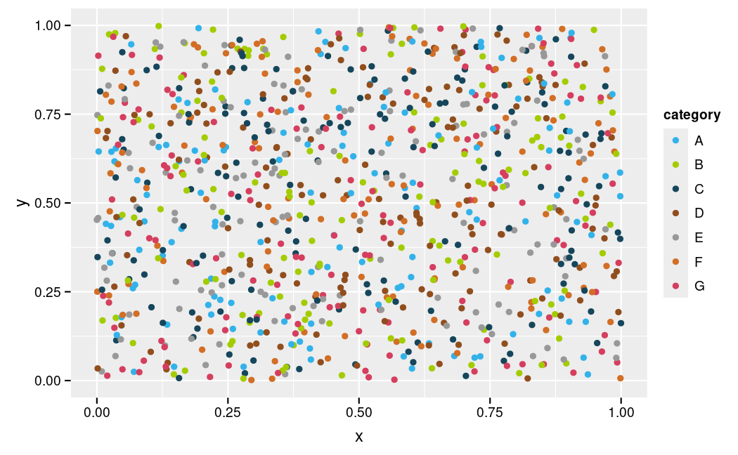
Coloured by a seven level categorical variable.
data.frame(
  x = runif(1e3), y = runif(1e3),
  category = sample(LETTERS[1:8], 1e3, replace = TRUE)
) |>
  ggplot(aes(x = x, y = y, colour = category)) +
  geom_jitter()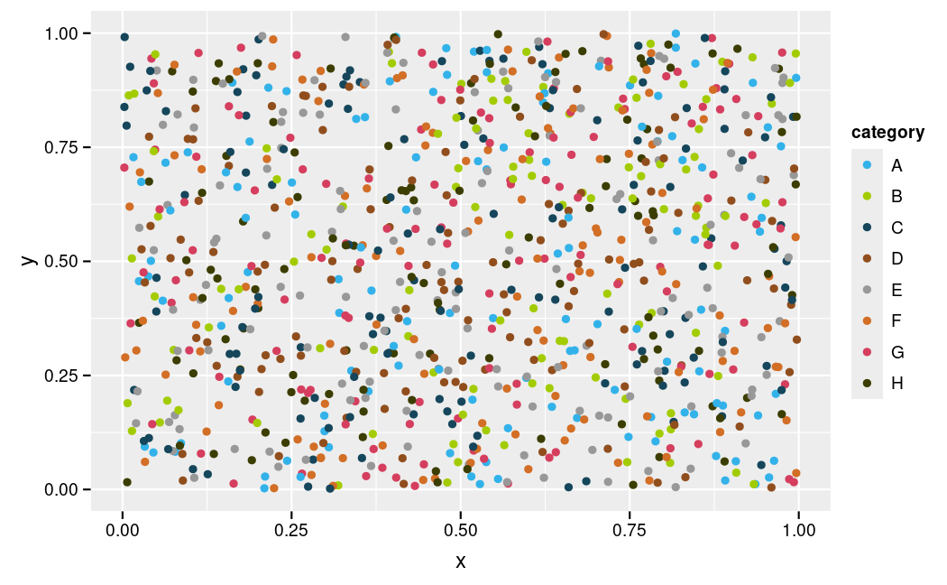
Coloured by an eight level categorical variable.
theme_elsevier()
Continuous variable
ggplot(diamonds, aes(x = carat, y = depth, colour = price)) +
  geom_point() +
  scale_colour_gradient()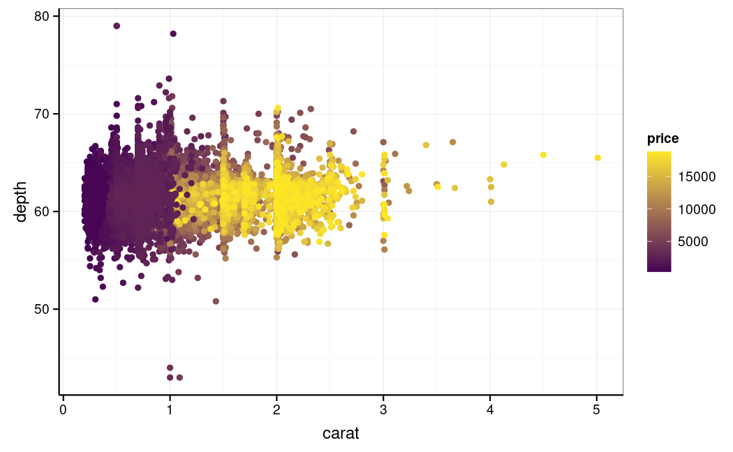
Coloured along a continuous variable.
ggplot(diamonds, aes(x = carat, y = depth, colour = price)) +
  geom_point() +
  scale_colour_gradient2(midpoint = 1e4)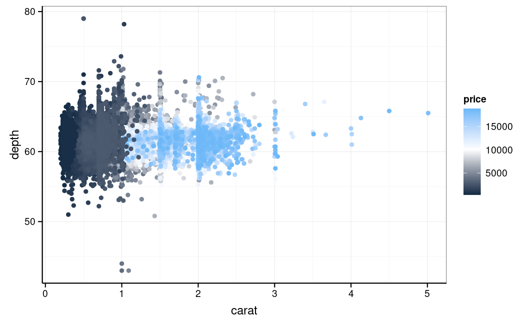
Coloured along a continuous variable using a gradient with midpoint.
Ordinal variable
ggplot(diamonds, aes(x = carat, y = depth, colour = cut)) +
  geom_point()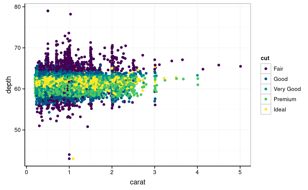
Coloured along an ordinal variable.
Categorical variable
Here we illustrate figures with a different number of categories. We choose for scatter plots with random x, y and category. This is the most difficult situation to distinguish the colours. Be careful when you use more than 5 colours.
data.frame(
  x = runif(1e3), y = runif(1e3),
  category = sample(LETTERS[1:2], 1e3, replace = TRUE)
) |>
  ggplot(aes(x = x, y = y, colour = category)) +
  geom_jitter()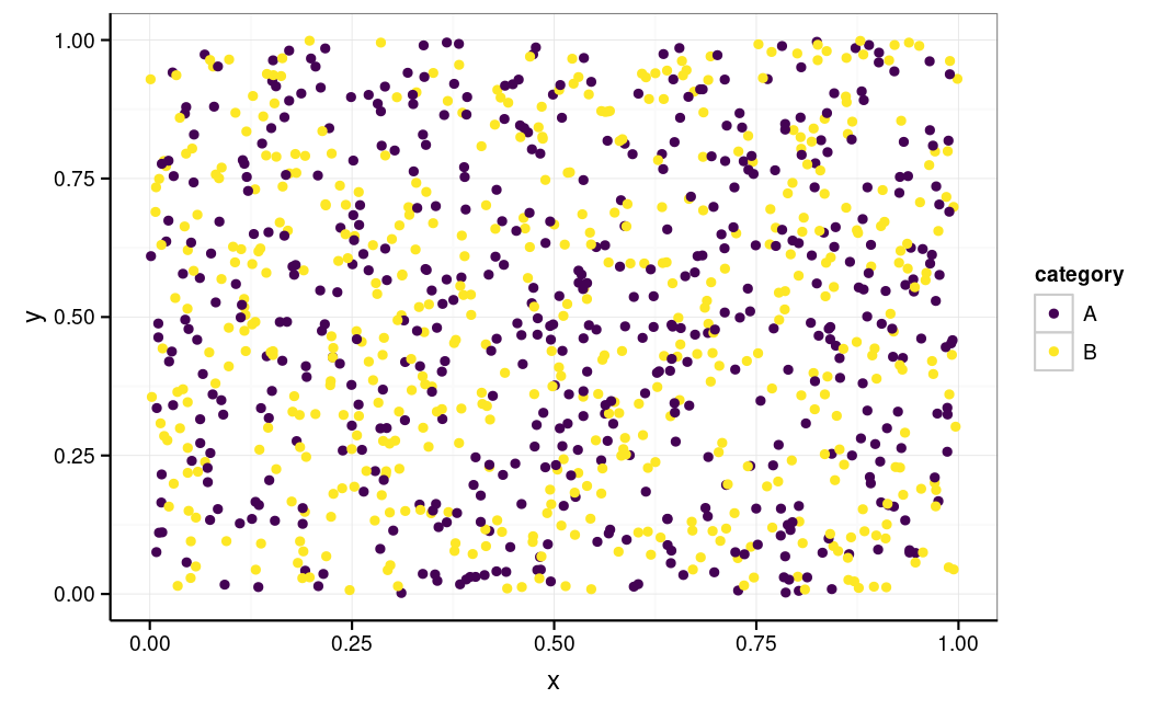
Coloured by a two level categorical variable.
data.frame(
  x = runif(1e3), y = runif(1e3),
  category = sample(LETTERS[1:3], 1e3, replace = TRUE)
) |>
  ggplot(aes(x = x, y = y, colour = category)) +
  geom_jitter()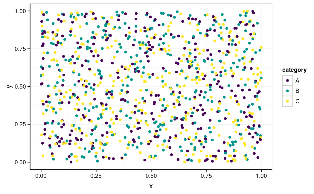
Coloured by a three level categorical variable.
data.frame(
  x = runif(1e3), y = runif(1e3),
  category = sample(LETTERS[1:4], 1e3, replace = TRUE)
) |>
  ggplot(aes(x = x, y = y, colour = category)) +
  geom_jitter()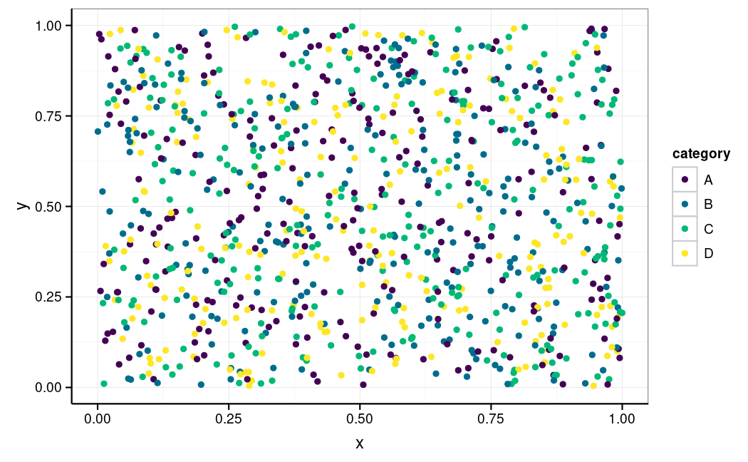
Coloured by a four level categorical variable.
data.frame(
  x = runif(1e3), y = runif(1e3),
  category = sample(LETTERS[1:5], 1e3, replace = TRUE)
) |>
  ggplot(aes(x = x, y = y, colour = category)) +
  geom_jitter()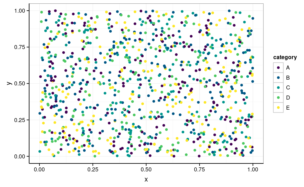
Coloured by a five level categorical variable.
data.frame(
  x = runif(1e3), y = runif(1e3),
  category = sample(LETTERS[1:6], 1e3, replace = TRUE)
) |>
  ggplot(aes(x = x, y = y, colour = category)) +
  geom_jitter()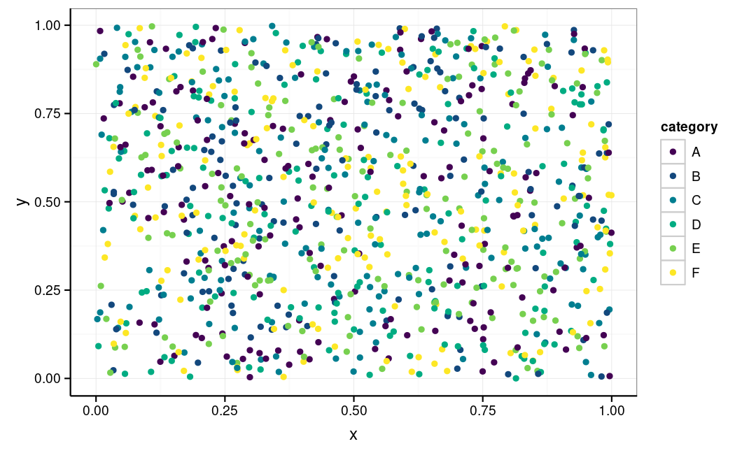
Coloured by a six level categorical variable.
data.frame(
  x = runif(1e3), y = runif(1e3),
  category = sample(LETTERS[1:7], 1e3, replace = TRUE)
) |>
  ggplot(aes(x = x, y = y, colour = category)) +
  geom_jitter()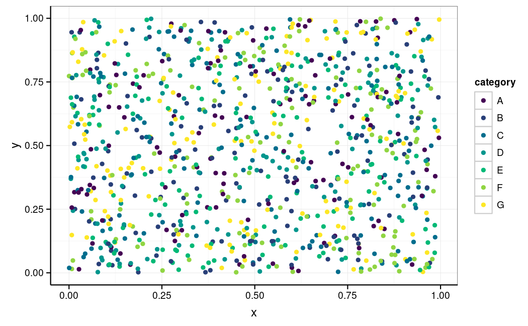
Coloured by a seven level categorical variable.
data.frame(
  x = runif(1e3), y = runif(1e3),
  category = sample(LETTERS[1:8], 1e3, replace = TRUE)
) |>
  ggplot(aes(x = x, y = y, colour = category)) +
  geom_jitter()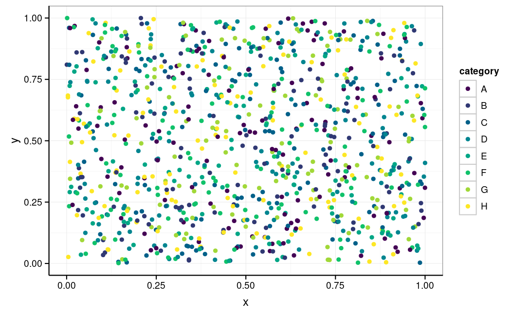
Coloured by an eight level categorical variable.