This document uses the National checklists and red lists for European butterflies dataset in this repository to create the tables and figures for Maes et al. (2019). It associated red list categories with numeric values to create weighted red list values per country and species. The source file for this document can be found here.

library(tidyverse)      # To do data science
library(tidylog)        # To provide feedback on dplyr functions
library(magrittr)       # To use %<>% pipes
library(here)           # To find files
library(janitor)        # To clean input data
library(gam)            # To work with generalized additive models

1 Read source data

The source data is maintained in a Google Spreadsheet and copied by src/dwc_mapping.Rmd to data/raw, from which we read it:

species_list <- read_csv(here::here("data", "raw", "taxa.csv"))
distribution <- read_csv(here::here("data", "raw", "distribution.csv"))
country_info <- read_csv(here::here("data", "raw", "regions.csv"))

2 Analysis data: taxon per country/island group

Create a dataframe of the taxa per country (= distributions) and associate with country information:

analysis_data <-
  distribution %>%
  left_join(country_info, by = "region_code")

See distinct red list categories:

analysis_data %>% distinct(rlc)

Associate a weighted red list value (see paper):

analysis_data %<>% mutate(rlc_numeric = recode(rlc, 
  RE = 100,
  CR = 80,
  EN = 50,
  VU = 30,
  NT = 20,
  LC = 1,
  DD = 1,
  Unknown = 1,
  
  R = 20, # Rare, used for Germany
  NE = 1,
  `LC/NE` = 1,
  NtA = NA_real_,
  NRLA = NA_real_
))

Exclude regional scientific names without an official scientific name:

analysis_data %<>% filter(!is.na(scientific_name)) # 11 rows

Remove duplicated rows (e.g. two local scientific names that were mapped to one):

analysis_data %<>% distinct(scientific_name, region_code, status, rlc, .keep_all = TRUE) # 17 rows

Show any remaining scientific_name + region_code duplicates that will be used in analysis:

analysis_data %>% filter(use == "y") %>% get_dupes(scientific_name, region_code) # 0 rows

Exclude non-countries, islands, and non-official scientific names. Keep island groups:

analysis_data %<>% filter(
  !is.na(country_code), # Exclude Europe, EU27, Macaronesia
  !str_detect(region_code, "MA_AZ_"), # Exclude Azores islands, keep island group MA_AZ
  !str_detect(region_code, "MA_CA_"), # Exclude Canary islands, keep island group MA_CA
  !str_detect(region_code, "MA_MA_") # Exclude Madeira islands, keep island group MA_MA
)

Only include taxa to be used for analysis (column use, based on breeding, regular migrant, regionally extinct, etc.):

analysis_data %<>% filter(use == "y")

Select useful fields and rename region_code to country_code (including countries + island groups):

analysis_data %<>%
  select(
    scientific_name,
    region_code,
    country_name,
    area,
    part_of_eu,
    status,
    endemic,
    rlc,
    rlc_numeric
  ) %>%
  rename(country_code = region_code)

Sort values by country, species:

analysis_data %<>% arrange(country_code, scientific_name)

Save file:

write_csv(analysis_data, here::here("data", "interim", "analysis_data.csv"), na = "")

3 Table 1: species per country

species_per_country <-
  analysis_data %>%
  group_by(country_name, country_code) %>%
  summarize(
    `n_species` = n_distinct(scientific_name),
    `n_endemic_species` = sum(!is.na(endemic))
  )

write_csv(species_per_country, here::here("reports", "species_per_country.csv"), na = "")

4 Figure 2: mean red list value per country (cRLV)

Linear model:

mean_rlc_per_country <-
  analysis_data %>%
    drop_na(rlc_numeric) %>%
  group_by(country_code) %>%
    do(
      lm(rlc_numeric ~ 1, data = .data) %>%
        predict.lm(
          ., 
            newdata = data.frame(rlc_numeric_a = 0, rlc_numeric_b = 1),
            interval = "confidence",
            level = 0.95
        ) %>%
        as.data.frame()
    )

Save data:

write.csv(mean_rlc_per_country, here::here("data", "interim", "mean_rlc_per_country.csv"), na = "")

Create plot:

mean_rlc_per_country_plot <- ggplot(mean_rlc_per_country, aes(x = reorder(country_code, -fit), y = fit)) + 
  geom_point() +
  geom_pointrange(aes(ymin = lwr, ymax = upr)) +
  xlab("CountryCode") +
  ylab("mRLV") + 
  geom_hline(yintercept = 50, size = 1, linetype = 1) + # colour = "red")
  geom_hline(yintercept = 30, size = 1, linetype = 2) + # , colour = "orange"
  geom_hline(yintercept = 20, size = 1, linetype = 3) + # , colour = "yellow"
  theme_bw()

ggsave(
  mean_rlc_per_country_plot,
  file = here::here("reports", "mean_rlv_per_country.jpg"),
  device = "jpeg",
  dpi = 300,
  height = 5,
  width = 10
)

mean_rlc_per_country_plot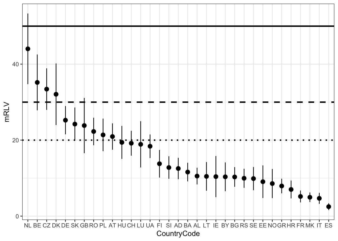

5 Table 3: weighted red list value per species (wsRLV)

We create this table by creating a number of dataframes summarizing information per scientific_name and then joining these together.

Create lookup of red list status for Europe and European Union.

# Use distribution df, since region_code = "EUR"/"EU27" is excluded from analysis data
rlc_eur <-
  distribution %>%
  filter(region_code == "EUR") %>%
  filter(use == "y") %>%
  select(scientific_name, rlc, endemic) %>%
  rename(rlc_eur = rlc, endemic_eur = endemic)

rlc_eu27 <-
  distribution %>%
  filter(region_code == "EU27") %>%
  filter(use == "y") %>%
  select(scientific_name, rlc, endemic) %>%
  rename(rlc_eu27 = rlc, endemic_eu27 = endemic)

Create lookup of endemic status:

endemic <-
  analysis_data %>%
  filter(!is.na(endemic)) %>%
  group_by(scientific_name) %>%
  summarize(
    endemic = paste(unique(endemic), collapse = "|")
  )

Create lookup of counts per species:

counts_eur <-
  analysis_data %>% # Contains all countries/island groups = Europe
  group_by(scientific_name) %>%
  summarize(
    n_species_eur = n(),
    n_rl_eur = sum(!is.na(rlc_numeric))
  )

Create lookup of counts per species in European Union:

counts_eu27 <-
  analysis_data %>%
  filter(!is.na(part_of_eu)) %>%
  group_by(scientific_name) %>%
  summarize(
    n_species_eu27 = n(),
    n_rl_eu27 = sum(!is.na(rlc_numeric))
  )

Create linear model for all species:

weighted_rlv_per_species <-
  analysis_data %>%
  group_by(scientific_name) %>%
  drop_na(rlc_numeric) %>%
  do(
    lm(rlc_numeric ~ 1, weights = sqrt(area), data = .) %>%
        predict.lm(
          .,
          newdata = data.frame(rlc_numeric_a = 0, rlc_numeric_b = 1),
            interval = "confidence",
            level = 0.95
        ) %>%
      as.data.frame()
    )

Save data:

write.csv(weighted_rlv_per_species, here::here("data", "interim", "weighted_rlv_per_species.csv"), na = "")

Create linear model for species in European Union:

weighted_rlv_per_species_eu27 <-
  analysis_data %>%
  drop_na(rlc_numeric) %>%
  filter(!is.na(part_of_eu)) %>%
  group_by(scientific_name) %>%
  do(
    lm(rlc_numeric ~ 1, weights = sqrt(area), data = .) %>%
        predict.lm(
          .,
          newdata = data.frame(rlc_numeric = 0, rlc_numeric = 1),
            interval = "confidence",
            level = 0.95
        ) %>%
      as.data.frame()
    )

Join information together with species list:

weighted_species_list <-
  species_list %>%
  left_join(rlc_eur, by = "scientific_name") %>%
  left_join(rlc_eu27, by = "scientific_name") %>%
  left_join(endemic, by = "scientific_name") %>%
  left_join(counts_eur, by = "scientific_name") %>%
  left_join(counts_eu27, by = "scientific_name") %>%
  left_join(
    weighted_rlv_per_species %>% select(scientific_name, fit) %>% rename(wsrlv_eur = fit),
    by = "scientific_name") %>%
  left_join(
    weighted_rlv_per_species_eu27 %>% select(scientific_name, fit) %>% rename(wsrlv_eu27 = fit),
    by = "scientific_name"
  )

Number of taxa should remain the same:

nrow(species_list) == nrow(weighted_species_list) # Expect TRUE

## [1] TRUE

Order by wsrlv_eur and select columns:

table3 <- weighted_species_list %>%
  arrange(desc(wsrlv_eur), desc(n_species_eur)) %>%
  select(
    scientific_name,
    endemic_eur,
    edge_of_range,
    wsrlv_eur,
    n_species_eur,
    n_rl_eur,
    rlc_eur,
    wsrlv_eu27,
    n_species_eu27,
    n_rl_eu27,
    rlc_eu27,
    habitats_directive,
    endemic
  ) %>%
  mutate(
    wsrlv_eur = round(wsrlv_eur, 2),
    wsrlv_eu27 = round(wsrlv_eu27, 2)
  )

Save file:

write_csv(table3, here::here("reports", "weighted_species_list.csv"), na = "")

6 Figure 3: correlation between srqt(area) and mean red list value

Calculate mean rlc per sqrt of area:

mean_rlc_sqrt_area <-
  analysis_data %>%
  mutate(
    rlc_numeric = round(rlc_numeric, 0),
    sqrt_area = sqrt(area/1000) # Divide by 1000
  ) %>%
  group_by(sqrt_area) %>%
  summarize(
    mean_rlc_numeric = mean(rlc_numeric, na.rm = TRUE)
  ) %>%
  filter(!is.na(mean_rlc_numeric))

Create plot:

mean_rlc_sqrt_area_plot <- ggplot(mean_rlc_sqrt_area, aes(x = sqrt_area, y = mean_rlc_numeric)) +
  geom_point() +
  geom_smooth(method = "lm", se = TRUE, colour = "black", formula = y ~ splines::ns(x, 1)) +
  theme_bw() +
  labs(x = "sqrt(area)", y = "mRLV") +
  theme(axis.text.x = element_text(face = "bold", size = 20), axis.text.y = element_text(face = "bold", size = 20)) +
  theme(axis.title = element_text(face = "bold", size = 22))

mean_rlc_sqrt_area_plot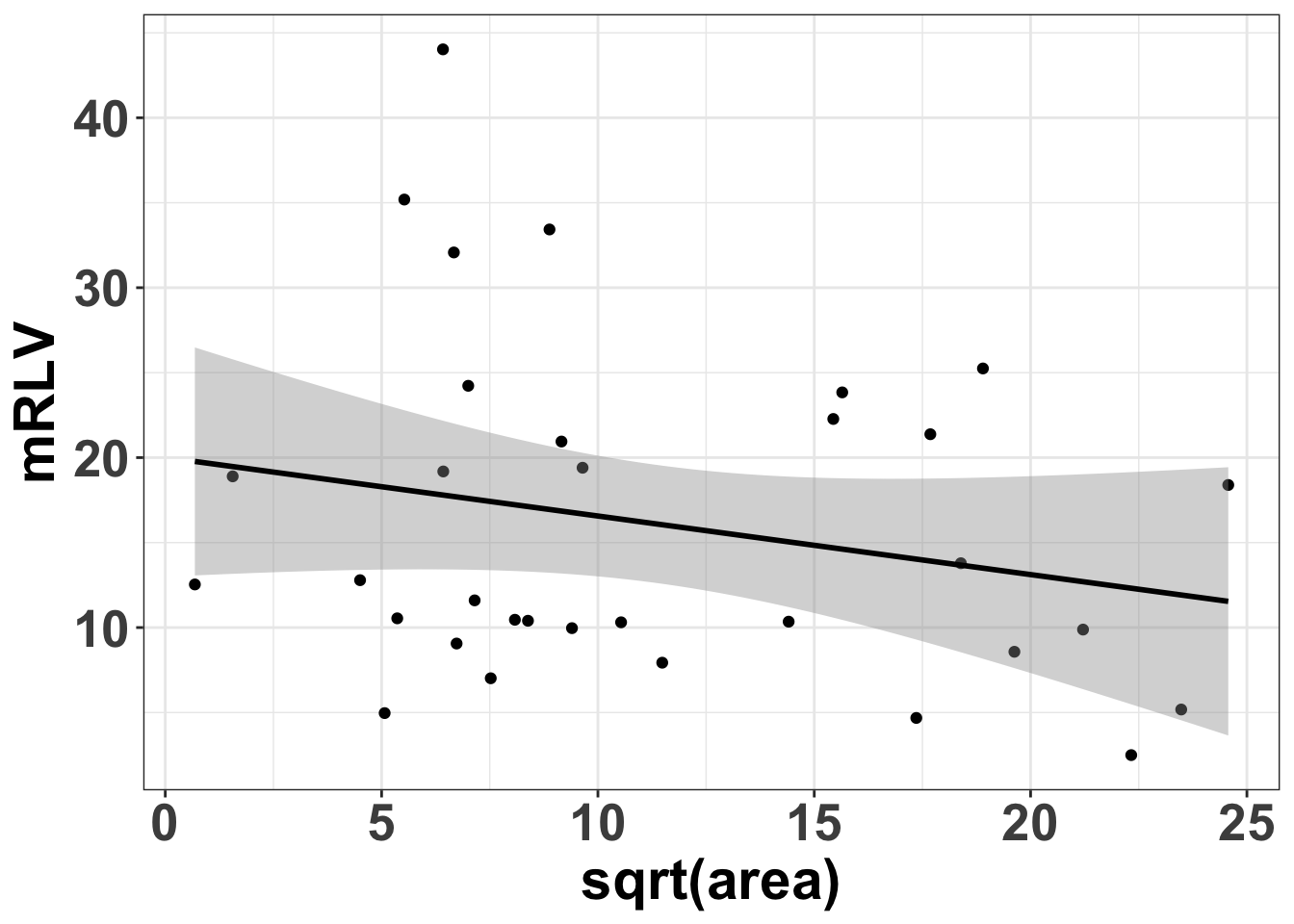

ggsave(mean_rlc_sqrt_area_plot, file = here::here("reports/mean_rlv_per_sqrt_area.jpg"), device = "jpeg", dpi = 300, height = 6, width = 10)

Integrating red lists

Dimitri Brosens

Dirk Maes

Peter Desmet