Basic Usage of grtsdb

Short introduction to Generalized Random Tessellation Stratified sampling (GRTS)

Quadrant recursive map

A key component of GRTS is translating 2D coordinates to 1D coordinates. This is done by quadrant recursive maps (Stevens and Olsen 1999, 2004). The map is split in 4 quadrants by splitting it halfway along the north-south axis and halfway along the east-west axis. This yields the level-1 split. Each quadrant of level-1 is in a similar way split into 4 sub quadrants. This yields 16 level-2 quadrants. This is recursively applied until each quadrant contains only one element or the dimensions of the quadrants are small enough. We give an example with three levels in the figure below.

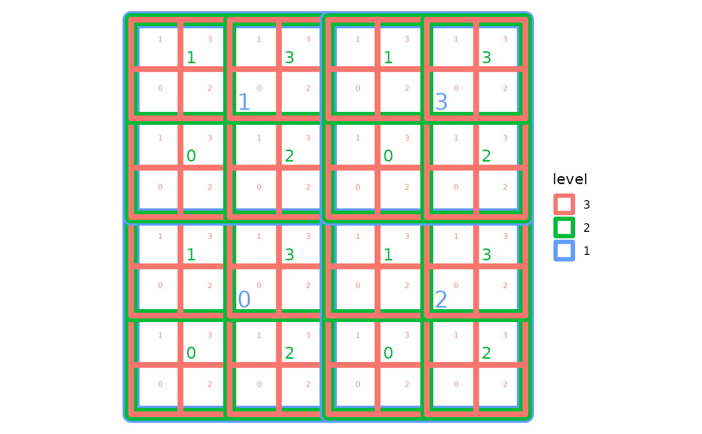
Example of a quandrant recursive map with three levels.

Reverse hierarchical ordering

We index each sub quadrant within a quadrant uniquely with the numbers 0, 1, 2 or 3 (figure above). The combination of this index with the indices of all lower levels gives a unique 1D address to each sub quadrant. The level-1 quadrants need only 1 index, the level-2 quadrants require 2 indices (level-1 and level-2), …

The 1D address can be though of as a base-4 number. In a typical hierarchical order we would use level-1 as the highest digit, level-2 as the next digit, and so on. The figure below shows the base-4 indices up to the third level. The background of each cell is coloured along a gradient of address (after conversion to base-10). The change in colour clearly reflects the level-1 structure. Adding 1 to the lowest digit (level-3 in this example), results in 3 out of 4 times in moving to a neighbouring cell. In other cases we would go to a cell in a neighbouring quadrant of a higher level. Thus the 1D address of neighbouring cells will be similar.

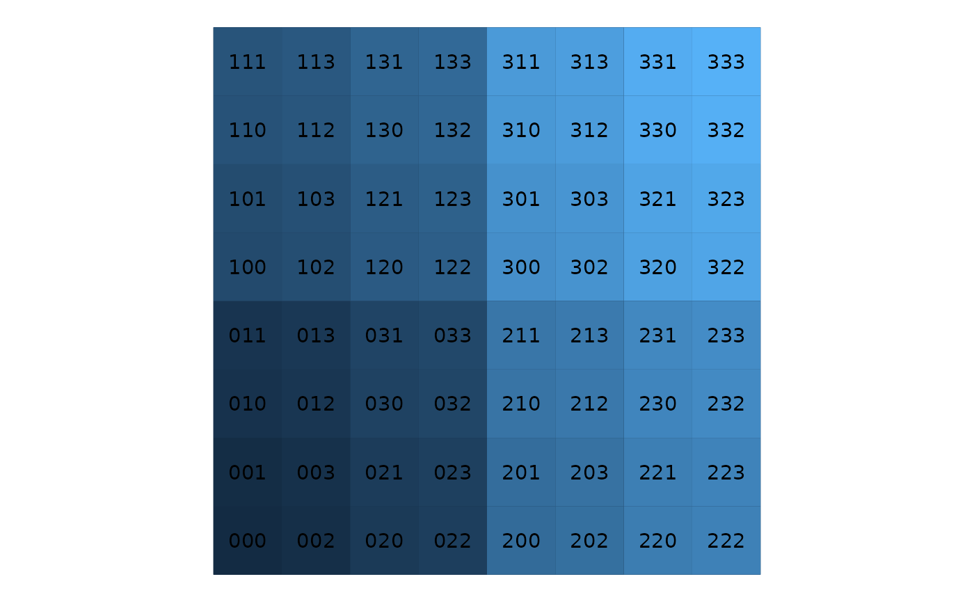
Example of a quandrant recursive map with three levels and base-4 indices.

The picture changes if we reverse the hierarchical order (fig below). Now we use level-1 as the lowest digit, level-2 as the second lowest digit, and so on.

Adding 1 to the lowest digit, will now result in moving to another level-1 quadrant. Hence the corresponding movement in 2D is always large.

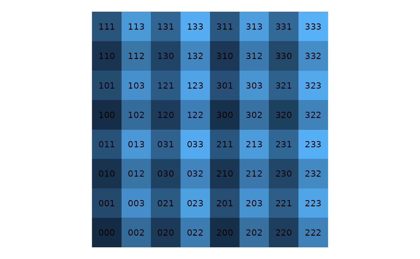
Example of a quandrant recursive map with three levels and reverse hierarchical base-4 indices.

Randomisation

The randomisation is done by permuting the indices of sub quadrant. Each split of a quadrant in 4 sub quadrants uses an independent random permutation.

Selection of the sample

The actual selection of the sample from the 1D address come in two flavours. The oldest flavour (Stevens and Olsen 1999) uses the normal hierarchical ordering. The actual sample uses a systematic sampling along the 1D addresses. It samples every \(N/n\) 1D address and uses a random start between \(0\) and \(N/n - 1\).

A more recent flavour Theobald et al. (2007), is based on the reverse hierarchical ordering. The actual sample uses the first \(n\) 1D addresses.

Benefits of the normal hierarchical order

• Unequal probability sampling is easy to implement. Consider each 1D address to be a line segment with length proportional to inclusion probability. Concatenate all line segments according to the order of the 1D address. Take a systematic sample along this concatenated line.

Benefits of the revese hierarchical order

• Replacement of drop-out samples is easy. Just take the next available 1D address.
• Repeated sampling in time is possible, provided the entire region is covered as a GRTS grid.

Main functionality of grtsdb

The most import functions of grtsdb are connect_db(), add_level() and extract_sample(). As grtsdb stores the randomised grid in a SQLite database, you first need to connect to such database with connect_db(). The default uses a file called grtsdb.sqlite in the current working directory. The function creates the file when it doesn’t exist. ":memory:" is a special type of “file”: the database is stored in memory and not on disk. Such database will be lost when the user disconnects. Databases stores on disk can be reused later.

library(grtsdb)
db_mem <- connect_db(":memory:")

The second step is the generate the randomised grids in the database using add_level(). This requires at least a connection to the database, the bounding box (\((x_0, x_1, y_0, y_1)\)) and the cell size of the grid (\(s\)). The function determines the largest grid required to cover the bounding box with a grid of the required cell size. Each dimension of this grid gets the same number of cells and this number will be a power of 2. We take the maximum of the number of grid cells in each dimension. The ceiling of a the \(\log\) base 2 of this maximum is the required level \(n\) because \(2^n\) will be larger or equal to this maximum.

\[n = \lceil\log_2\frac{\max(x_1 - x_0, y_1 - y_0)}{s}\rceil\]

bbox <- rbind(
  x = c(10000, 50000),
  y = c(-25000, 10000)
)
cellsize <- 1000
add_level(bbox = bbox, cellsize = cellsize, grtsdb = db_mem)
#> Required number of levels: 6
#> Adding level 1: create table, add coordinates, calculate ranking
#> Adding level 2: create table, add coordinates, calculate ranking
#> Adding level 3: create table, add coordinates, calculate ranking
#> Adding level 4: create table, add coordinates, calculate ranking
#> Adding level 5: create table, add coordinates, calculate ranking
#> Adding level 6: create table, add coordinates, calculate ranking

Now we are ready to take a sample using extract_sample() on the database. The result is a data frame containing the coordinates (centroids of the grid cell) and their ranking. The samplesize arguments defines to number of grid cells to return. The grid is on-the-fly defined by the bounding box and the cell size. The function returns the grid cells within the bounding box and with the lowest ranking. Hence the ranking seems to “skip” some of the ranking values.

extract_sample(
  grtsdb = db_mem, samplesize = 5, bbox = bbox, cellsize = cellsize
)
#> Creating index for level 6. May take some time...
#>  Done.
#>     x1c    x2c ranking
#> 1 24500   8000       1
#> 2 29500 -24000       4
#> 3 20500 -17000       8
#> 4 47500   7000      11
#> 5 45500 -20000      14

The last step is discard the grid cells outside of the sampling frame. Therefore the user needs to extract more grid cells within the bounding box than needed. The required oversampling rate is slightly larger than the ratio between the area of the bounding box and the area of the sampling frame. If the area of the bounding box is twice the area of the sampling frame, then extract at least twice the final sample size. Keep grid cells with smallest ranking in case you end up with too many grid cells in the sampling frame.

Because the randomisation is stored in the database, rerunning extract_sample() on the same database with the same argument will yield the same sample. The example below is a rerun with a larger samplesize. Note that the first rows are identical. The sample is supplemented with additional grid cells. Internally the bounding box is centred with the full grid with \(2^n\) cells in each dimension. As a result, shifting the bounding box will yield the same shift in the sample.

extract_sample(
  grtsdb = db_mem, samplesize = 10, bbox = bbox, cellsize = cellsize
)
#>      x1c    x2c ranking
#> 1  24500   8000       1
#> 2  29500 -24000       4
#> 3  20500 -17000       8
#> 4  47500   7000      11
#> 5  45500 -20000      14
#> 6  45500   3000      15
#> 7  10500 -17000      16
#> 8  27500  -2000      17
#> 9  28500 -23000      24
#> 10 45500 -14000      30

The actual process of selecting the grid cells with a sampling frame is not implemented in grtsdb. This is a deliberate choice as it keeps the number of dependencies of the package minimal. In case of the 2D sampling frame, we recommend the sf package.

Nested samples

Note that the output of add_level() mentions adding several layers. This is because grtsdb stores the randomisation at every level. Level 1 being only 4 quadrants (\(4 ^ 1\)), level 2 has 16 (\(4 ^ 2\)) quadrants, … This implies that is straightforward to generate nested samples with different resolutions as long as the ratio between the resolutions is a power of two. The match is not perfect unless the bounding box is square and each dimension contains a power of 2 cells.

fine <- extract_sample(
  grtsdb = db_mem, samplesize = 20, bbox = bbox, cellsize = cellsize
)
coarse <- extract_sample(
  grtsdb = db_mem, samplesize = 20, bbox = bbox, cellsize = cellsize * 4
)
#> Creating index for level 4. May take some time...
#>  Done.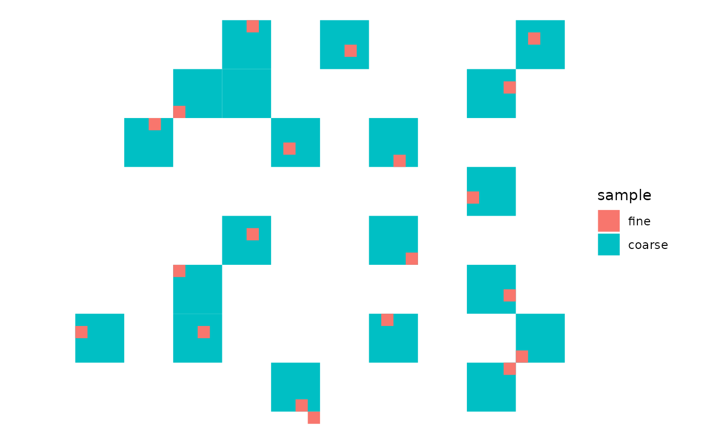

Example of two samples with nested grids.

Repeated samples

Image a long term monitoring of a number of sites within a given sampling frame. We can use a GRTS sample to get a spatially balanced selection. But what if the sampling frame changes in the future? E.g. the sampling frame is the set of all forests in a country. Deforested sites will leave the sampling frame while afforested sites will enter the sampling frame. Over time some of the early sampled sites might no longer be part of the sampling frame. We want to remove those sites from the sample and replace them with “fresh” sites. But what to do with the afforested sites that entered the sampling frame?

One solution would be to draw every so often a new an independent GRTS sample using the updated sampling frame. This would eliminate sites not longer in the sampling frame and allow new sites in the sampling frame to enter the sample. However, this brakes building a time series at sites that remain in the sampling frame.

We suggest to store the grtsdb database so the user can extract the same sample again in the future. This extraction is stable as long as we use the same database, with the same bounding box and cell size. The thing that changes is the sampling frame. Hence grid cells with low ranking outside the new sampling frame will be discarded. And new sites in the sampling frame enter the selection when they have a low ranking. The proportion of stable sites (sites both in the old and the new sample) will be proportional to the stable area (area in both the old and new sampling frame).

n-dimensional GRTS

The original GRTS algorithm handles only 2D problems. We altered the algorithm so it can handle n-D problems.

Here is an example of a 1D problem.

#> Required number of levels: 6
#> Adding level 1: create table, add coordinates, calculate ranking
#> Adding level 2: create table, add coordinates, calculate ranking
#> Adding level 3: create table, add coordinates, calculate ranking
#> Adding level 4: create table, add coordinates, calculate ranking
#> Adding level 5: create table, add coordinates, calculate ranking
#> Adding level 6: create table, add coordinates, calculate ranking
#> Creating index for level 6. May take some time...
#>  Done.
#>    x1c ranking
#> 1 0.47       0
#> 2 0.75       1
#> 3 0.89       3
#> 4 0.19       4
#> 5 0.65       5

The next examples works on a 3D problem. Here we used cells with unequal size for different dimensions. Keep in mind that the “spatial” balance only holds for the rescaled version, assuming equal cell sizes in every dimension.

#> Required number of levels: 4
#> Adding level 1: create table, add coordinates, calculate ranking
#> Adding level 2: create table, add coordinates, calculate ranking
#> Adding level 3: create table, add coordinates, calculate ranking
#> Adding level 4: create table, add coordinates, calculate ranking
#> Creating index for level 4. May take some time...
#>  Done.
#>    x1c  x2c x3c ranking
#> 1 0.25 0.75 0.0      18
#> 2 0.85 0.75 0.2      19
#> 3 0.55 0.25 0.0      20
#> 4 0.55 0.35 0.6      22
#> 5 0.35 0.35 1.0      39

Stevens, Don L., and Anthony R. Olsen. 1999. “Spatially Balanced Sampling of Natural Resources.” Journal of the American Statistical Association 99: 262–78.

———. 2003. “Variance Estimation for Spatially Balanced Samples of Environmental Resources.” Environmetrics 14 (6): 593–610.

———. 2004. “Spatially Balanced Sampling of Natural Resources.” Journal Of The American Statistical Association 99 (465): 262–78. https://doi.org/10.1198/016214504000000250.

Theobald, David, Don Stevens, Denis White, N. Urquhart, Anthony Olsen, and John Norman. 2007. “Using GIS to Generate Spatially Balanced Random Survey Designs for Natural Resource Applications.” Environmental Management 40 (1): 134–46. https://doi.org/10.1007/s00267-005-0199-x.