How to retrieve data from the Meetnetten database

Introduction

The Flemish species monitoring programme Meetnetten.be consists of a set of monitoring schemes for priority species in Flanders, the northern part of Belgium. The monitoring programme is a collaboration between the Nature and Forest Research Institute (INBO), the Nature and Forest Agency (ANB), the NGO Natuurpunt and many volunteers.

Each monitoring scheme consists of a number of monitoring sites at which target species are counted using a standardized protocol. The count data is stored in the Meetnetten database which is maintained by INBO. We present some functions to easily access the data from the Meetnetten database.

Aim

We make functions available to query data directly from the Meetnetten database. This avoids writing your own queries.

We have provided functions to query

monitoring schemes included in the species monitoring programme
locations and sublocations (for example different sections of a transect) of the monitoring schemes
visits (count events)
observations

Packages and connection

The main functions that we will use in this tutorial all start with get_meetnetten_*. These functions are made available by loading the inbodb package.

library(inbodb)
library(dplyr)
library(sf)
library(ggplot2)

These functions will only work for people with access to the INBO network. As an INBO employee, you should make sure you have read rights for the INBO Data Warehouse server, otherwise place an ICT-call.

The following R-code can be used to establish a connection to the Meetnetten database:

con <- connect_inbo_dbase("S0008_00_Meetnetten")

Functionality

Information on monitoring schemes

The function get_meetnetten_schemes() gives an overview per species group of all monitoring schemes included in Meetnetten and the protocols that are applied in the monitoring schemes.

In most cases, a monitoring scheme is dedicated to one target species and the monitoring scheme is named after the target species. In some cases, a monitoring scheme has several target species, such as the Algemene Broedvogelmonitoring Vlaanderen.

scheme_info <- get_meetnetten_schemes(con) %>%
  as_tibble()

scheme_info
#> # A tibble: 89 × 3
#>    species_group scheme        protocol                        
#>    <chr>         <chr>         <chr>                           
#>  1 amfibieën     Boomkikker    Amfibieën - Larven en metamorfen
#>  2 amfibieën     Boomkikker    Padden en kikkers - Roepkoren   
#>  3 amfibieën     Heikikker     Heikikker - DNA eitjes          
#>  4 amfibieën     Kamsalamander Amfibieën - Fuiken              
#>  5 amfibieën     Kamsalamander Amfibieën - Larven en metamorfen
#>  6 amfibieën     Knoflookpad   Amfibieën - Larven en metamorfen
#>  7 amfibieën     Knoflookpad   Knoflookpad - Roepkoren         
#>  8 amfibieën     Poelkikker    Padden en kikkers - Roepkoren   
#>  9 amfibieën     Poelkikker    Poelkikker - DNA larven         
#> 10 amfibieën     Rugstreeppad  Rugstreeppad - Transect         
#> # ℹ 79 more rows

Locations and sublocation of monitoring schemes

Each monitoring scheme consists of a fixed set of locations where the target species is/are counted on a regular basis. Some locations are subdivided in sublocations. This is, for example, the case for most butterfly monitoring schemes, where the sublocations represent the 50 meter sections of a transect.

The function get_meetnetten_locations() returns the locations and the sublocations for one or several monitoring scheme. It returns a list of two sf objects: main_locations and sublocations.

In the following example we select the locations and sublocations of the Argusvlinder (Lasiommata megera) monitoring scheme.


locations <- get_meetnetten_locations(con,
                                      scheme_name = "Argusvlinder")

main_locations <- locations$main_locations

sublocations <- locations$sublocations

Let’s have a look at the main_locations.

main_locations %>%
  head(5)
#> Simple feature collection with 5 features and 5 fields
#> Geometry type: POLYGON
#> Dimension:     XY
#> Bounding box:  xmin: 2.830468 ymin: 50.73131 xmax: 5.903817 ymax: 51.29184
#> Geodetic CRS:  WGS 84
#> # A tibble: 5 × 6
#>   species_group scheme    location is_sample is_active                      geom
#>   <chr>         <chr>     <chr>    <lgl>     <lgl>                 <POLYGON [°]>
#> 1 dagvlinders   Argusvli… Altenbr… TRUE      TRUE      ((5.800028 50.74765, 5.7…
#> 2 dagvlinders   Argusvli… Arenber… TRUE      TRUE      ((4.198335 51.27037, 4.2…
#> 3 dagvlinders   Argusvli… Blankaa… TRUE      TRUE      ((2.860811 50.98385, 2.8…
#> 4 dagvlinders   Argusvli… Blankaa… TRUE      TRUE      ((2.832082 50.98425, 2.8…
#> 5 dagvlinders   Argusvli… Boender… FALSE     TRUE      ((5.902601 50.73487, 5.9…

Two variables need some further explanation:

is_sample. For more common species, a random sample is drawn from all locations in Flanders where the target species occurs. For location that are selected is_sample = TRUE. Locations that are not selected, indicated by is_sample = FALSE, can be counted optionally.
is_active. When is_active = FALSE, the location is no longer counted. This is the case when the location appears to be inaccessible or when the target species does not occur at the location any more. However, most often these inactive locations where counted in previous years. So the the database also contains observations for (currently) inactive locations.

Next, let’s have a look at the sublocations of the location Arenbergpolder. The locations consists of 14 sections. Note that we only show the active (is_active = TURE) sublocations.

sublocations_show <- sublocations %>%
  filter(location == "Arenbergpolder") %>%
  filter(is_active)

sublocations_show
#> Simple feature collection with 14 features and 5 fields
#> Geometry type: LINESTRING
#> Dimension:     XY
#> Bounding box:  xmin: 4.202355 ymin: 51.27479 xmax: 4.217328 ymax: 51.28715
#> Geodetic CRS:  WGS 84
#> # A tibble: 14 × 6
#>    species_group scheme location sublocation is_active                      geom
#>  * <chr>         <chr>  <chr>    <chr>       <lgl>              <LINESTRING [°]>
#>  1 dagvlinders   Argus… Arenber… Sectie1     TRUE      (4.202355 51.27479, 4.20…
#>  2 dagvlinders   Argus… Arenber… Sectie10    TRUE      (4.214129 51.28617, 4.21…
#>  3 dagvlinders   Argus… Arenber… Sectie11    TRUE      (4.214694 51.28647, 4.21…
#>  4 dagvlinders   Argus… Arenber… Sectie12    TRUE      (4.21528 51.28671, 4.215…
#>  5 dagvlinders   Argus… Arenber… Sectie13    TRUE      (4.215934 51.28693, 4.21…
#>  6 dagvlinders   Argus… Arenber… Sectie14    TRUE      (4.216612 51.28707, 4.21…
#>  7 dagvlinders   Argus… Arenber… Sectie2     TRUE      (4.202677 51.27517, 4.20…
#>  8 dagvlinders   Argus… Arenber… Sectie3     TRUE      (4.203014 51.27557, 4.20…
#>  9 dagvlinders   Argus… Arenber… Sectie4     TRUE      (4.203358 51.27599, 4.20…
#> 10 dagvlinders   Argus… Arenber… Sectie5     TRUE      (4.203695 51.27636, 4.20…
#> 11 dagvlinders   Argus… Arenber… Sectie6     TRUE      (4.204002 51.27675, 4.20…
#> 12 dagvlinders   Argus… Arenber… Sectie7     TRUE      (4.204346 51.27718, 4.20…
#> 13 dagvlinders   Argus… Arenber… Sectie8     TRUE      (4.213335 51.28542, 4.21…
#> 14 dagvlinders   Argus… Arenber… Sectie9     TRUE      (4.213685 51.28582, 4.21…

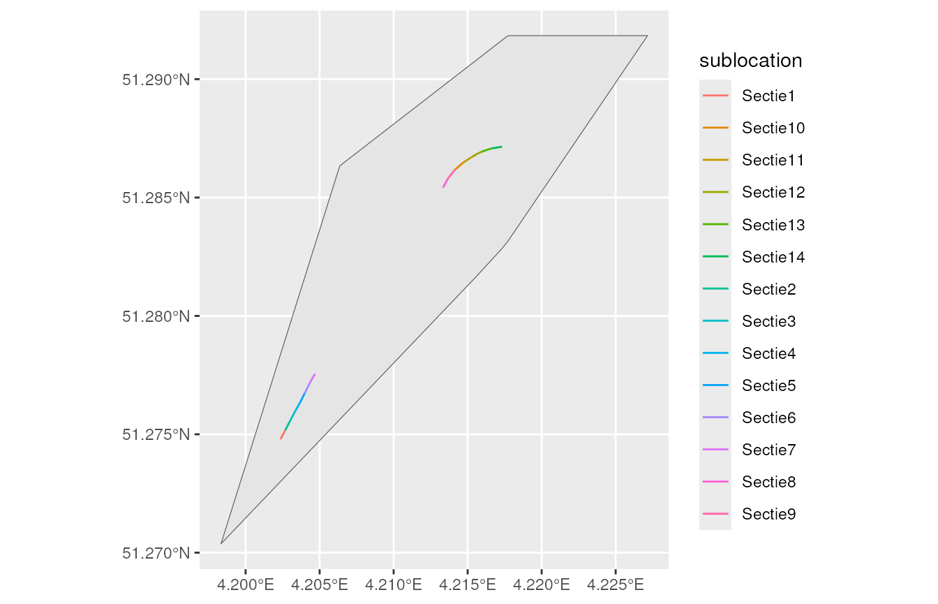
Below we show a basic map of the locations and sublocations. The location is the wider area where the target species occurs. The sublocations indicate where the target species is counted.


main_location_show <- main_locations %>%
  filter(location == "Arenbergpolder")

ggplot(sublocations_show) +
  geom_sf(data = main_location_show) +
  geom_sf(aes(colour = sublocation))

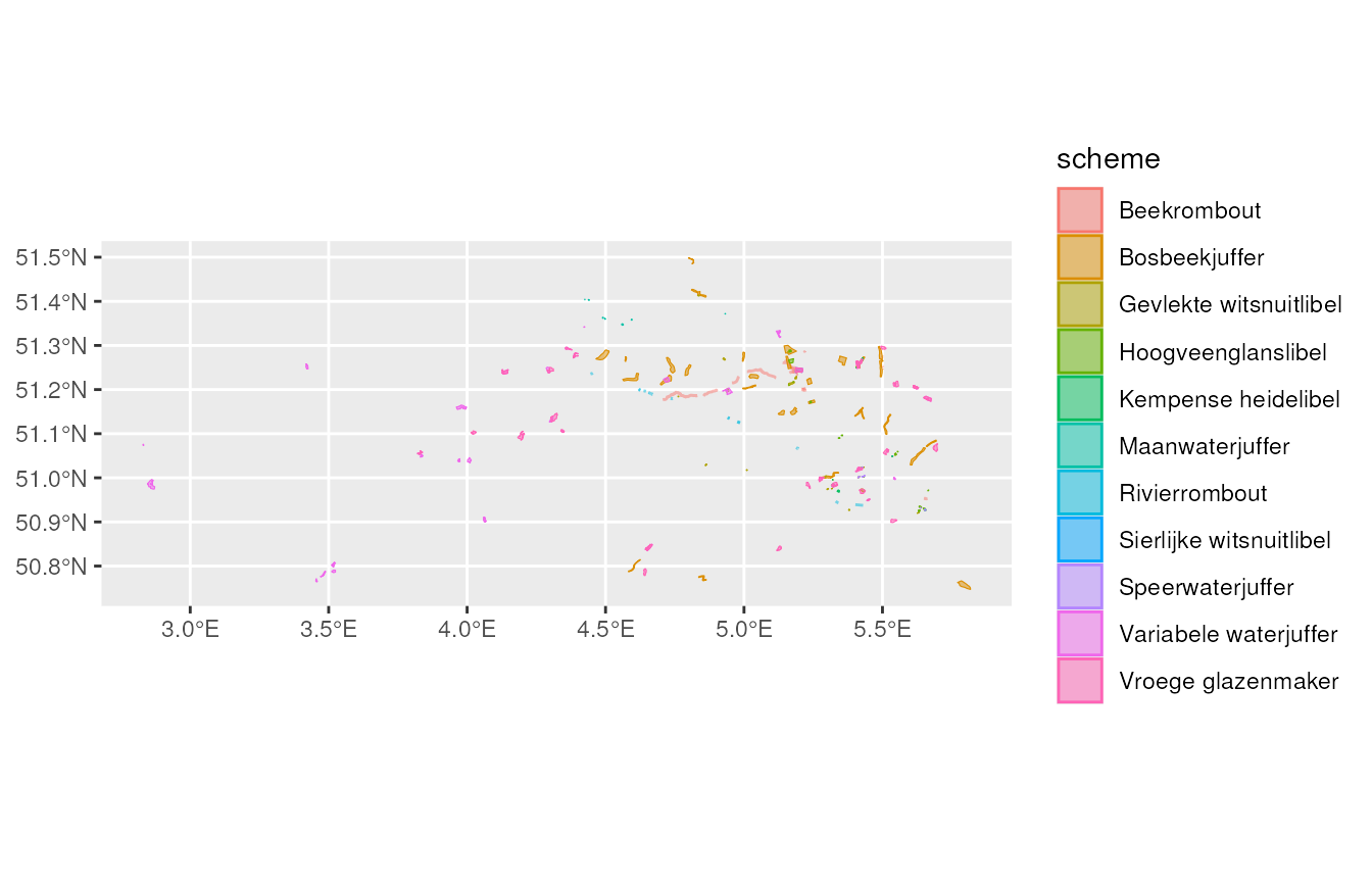
We can also select and plot all locations from the dragonfly (in Dutch libellen) monitoring schemes.

# get locations for a specific species_group
locations_dragonflies <- get_meetnetten_locations(con,
                                                  species_group = "libellen")


locations_dragonflies$main_locations %>%
  ggplot() +
  geom_sf(aes(fill = scheme, colour = scheme), alpha = 0.5)

Visits

The function get_meetnetten_visits() returns all visits (count events) for one or more monitoring schemes.

Below we select all visits for the location Arenbergpolder of the Argusvlinder monitoring scheme. We see that in most years the location is counted 6 times per year as demanded by the monitoring protocol.


visits <- get_meetnetten_visits(con,
                                scheme_name = "Argusvlinder",
                                collect = TRUE)

visits %>%
  filter(location == "Arenbergpolder") %>%
  select(location, visit_id, start_date,
         start_time, visit_status)
#> # A tibble: 33 × 5
#>    location       visit_id start_date start_time visit_status    
#>    <chr>             <int> <date>     <chr>      <chr>           
#>  1 Arenbergpolder      262 2016-05-13 09:55:00   Conform protocol
#>  2 Arenbergpolder      263 2016-05-21 13:45:00   Conform protocol
#>  3 Arenbergpolder      264 2016-05-26 13:45:00   Conform protocol
#>  4 Arenbergpolder      479 2016-07-20 08:50:00   Conform protocol
#>  5 Arenbergpolder      480 2016-08-09 09:25:00   Conform protocol
#>  6 Arenbergpolder      481 2016-08-17 12:05:00   Conform protocol
#>  7 Arenbergpolder     1517 2017-04-21 13:08:00   Conform protocol
#>  8 Arenbergpolder     1080 2017-05-10 15:38:00   Conform protocol
#>  9 Arenbergpolder     1518 2017-05-17 15:00:00   Conform protocol
#> 10 Arenbergpolder     1661 2017-08-02 12:47:00   Conform protocol
#> # ℹ 23 more rows

Use ?get_meetnetten_visits to get more information on the variables that are returned by the function.

Observations

The function get_meetnetten_observations() provides all observations for one or more monitoring scheme.

Let’s select all observations from one visit at the Arenbergpolder location of the Argusvlinder monitoring scheme, by applying a filter based on the variable visit_id.


observations <- get_meetnetten_observations(con,
                                            scheme_name = "Argusvlinder",
                                            collect = FALSE) %>%
  filter(visit_id == 1080) %>%
  collect()

First we take a look at the observation of the target species.


observations %>%
  filter(target_species) %>%
  select(location, sublocation, start_date,
         scientific_name, count)
#> # A tibble: 14 × 5
#>    location       sublocation start_date scientific_name   count
#>    <chr>          <chr>       <date>     <chr>             <int>
#>  1 Arenbergpolder Sectie4     2017-05-10 Lasiommata megera     1
#>  2 Arenbergpolder Sectie5     2017-05-10 Lasiommata megera     0
#>  3 Arenbergpolder Sectie6     2017-05-10 Lasiommata megera     1
#>  4 Arenbergpolder Sectie1     2017-05-10 Lasiommata megera     1
#>  5 Arenbergpolder Sectie2     2017-05-10 Lasiommata megera     0
#>  6 Arenbergpolder Sectie3     2017-05-10 Lasiommata megera     0
#>  7 Arenbergpolder Sectie8     2017-05-10 Lasiommata megera     0
#>  8 Arenbergpolder Sectie7     2017-05-10 Lasiommata megera     0
#>  9 Arenbergpolder Sectie9     2017-05-10 Lasiommata megera     0
#> 10 Arenbergpolder Sectie10    2017-05-10 Lasiommata megera     0
#> 11 Arenbergpolder Sectie12    2017-05-10 Lasiommata megera     0
#> 12 Arenbergpolder Sectie13    2017-05-10 Lasiommata megera     0
#> 13 Arenbergpolder Sectie14    2017-05-10 Lasiommata megera     0
#> 14 Arenbergpolder Sectie11    2017-05-10 Lasiommata megera     0

Optionally observers can also record non target species that can be counted using the same protocol.

The code below provides the total number of individuals per species, including the non target species, that were counted in one visit at the Arenbergpolder location.


observations %>%
  group_by(start_date, target_species, name_nl, scientific_name) %>%
  summarise(count_total = sum(count)) %>%
  ungroup()
#> `summarise()` has grouped output by 'start_date', 'target_species', 'name_nl'.
#> You can override using the `.groups` argument.
#> # A tibble: 6 × 5
#>   start_date target_species name_nl             scientific_name      count_total
#>   <date>     <lgl>          <chr>               <chr>                      <int>
#> 1 2017-05-10 FALSE          Bruin blauwtje      Aricia agestis                 2
#> 2 2017-05-10 FALSE          Hooibeestje         Coenonympha pamphil…          10
#> 3 2017-05-10 FALSE          Klein geaderd witje Pieris napi                    3
#> 4 2017-05-10 FALSE          Klein koolwitje     Pieris rapae                   1
#> 5 2017-05-10 FALSE          Kleine vuurvlinder  Lycaena phlaeas                3
#> 6 2017-05-10 TRUE           Argusvlinder        Lasiommata megera              3

Use ?get_meetnetten_observations to get more information on the variables that are returned by the function.

An important note: before you start analysing the data from a certain monitoring scheme, it is important to know how the monitoring schemes were designed and how the data is organised. So don’t forget to check the monitoring protocol (available on the INBO website).

Closing the connection

Close the connection when done

dbDisconnect(con)
rm(con)

Data policy

Since many of the target species are sensitive species, we do not publicly make available the exact location of the observations. Location information is generalized to 1, 5 or 10 km Universal Transverse Mercator (UTM) grid cells, when publishing the data on GBIF. The generalisation rules are the same as in waarnemingen.be.

Please respect this policy when you publish results based on the Meetnetten data. Also please contact info@meetnetten.be before publishing results. This way we can check if the publication complies with the data policy as agreed by the different project parters of Meetnetten.

Toon Westra, Frederic Piesschaert

2024-06-25